3.2. Catapult System Tutorial (AutoDesign)

3.2.1. Outline of Tutorial Sample B

Model

Description

Sample_B

Catapult System Design Problem: The design goal is that a ball, thrown by catapult system, should pass through a tight cylinder. This problem is a difficult problem because the dynamic analysis gives noisy response, which is a typical characteristic of dynamic response optimization. This sample result shows why AutoDesign is a good choice for dynamic system optimization. Key Point: Study the Variable Equation and Expression for defining the velocity and the position error when the ball passes through the target position.

3.2.2. Catapult System Design Problem

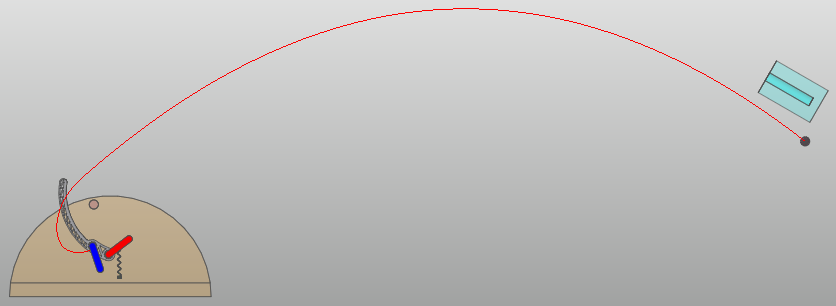
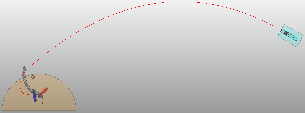
Figure 3.37 shows a catapult with a curved arm, which throws a ball using a target. Certain aspects of the catapult can be changed to aim the catapult. These are the angle of the front link at start position and the mount point of the main spring to the front link. As the engineer, your goal is to control these parameters such that the ball will not only arrive at the mouth of the target but will also do so with the correct angle of attack which will allow the ball to go inside.

The model supplied with this tutorial will have all of the geometry and joint modeling complete but are not ready for optimization. In this tutorial sample, you will learn how to prepare this model for design optimization.

Open files related inSample-B
Sample	<InstallDir>\Help\Tutorial\AutoDesign\CatapultSystem\Examples\Sample_B.rdyn
Solution	<InstallDir>\Help\Tutorial\AutoDesign\CatapultSystem\Solutions\Sample_B.rdyn

Note

If you change the file path at discretion, it can be located in any folder that you specify.

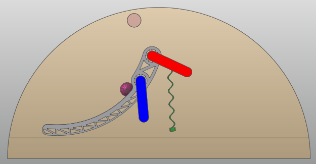
Figure 3.37 Catapult system

3.2.3. Loading the Model and Viewing the Animation

3.2.3.1. To load the base model and view the animation:

1. On your Desktop, double-click the RecurDyn icon. RecurDyn starts and the Start RecurDyn dialog box appears.

2. Close Start RecurDyn dialog box. You will use an existing model.

3. In the toolbar, click the Open tool and select Sample_B.rdyn from the same directory where this tutorial is located.

   The catapult appears in the modeling window.

4. Run Simulate.

5. Click Play.

   The trajectory of the ball should appear as shown below. The contact between the ball and the target has been disabled so that it does not interfere with the design optimization results. Also, an inplane joint was added to remove out-of-plane movement of the ball in the z-direction, as a small amount of this was inevitable due to the tessellation of the catapult arm’s track surface. The main focus of the model is on the ball’s movement in the x- and y-directions.
   

3.2.4. Design Variables

The design variables will be the factors of the model which you can control. Figure 3.38 is a diagram showing these factors on the model.

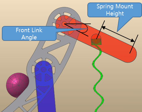
Figure 3.38 Two design variables

Front link angle is defined as the angle of the front link from horizontal, measured at the rear pivot point. As the front link angle is varied, the rear pivot point remains stationary while the front pivot point moves to accommodate the angle change.

Spring mount height is the distance between the spring mount point and the front pivot and is expressed as a fraction of the entire link length (the distance between the front and rear pivots).

3.2.4.1. Exercising the Model

You will now explore how changing the design variables affects the ball’s trajectory. In this model, the design variables will be linked to parametric values, so for now you will actually vary the parametric values, instead.

3.2.4.1.1. To exercise the model:

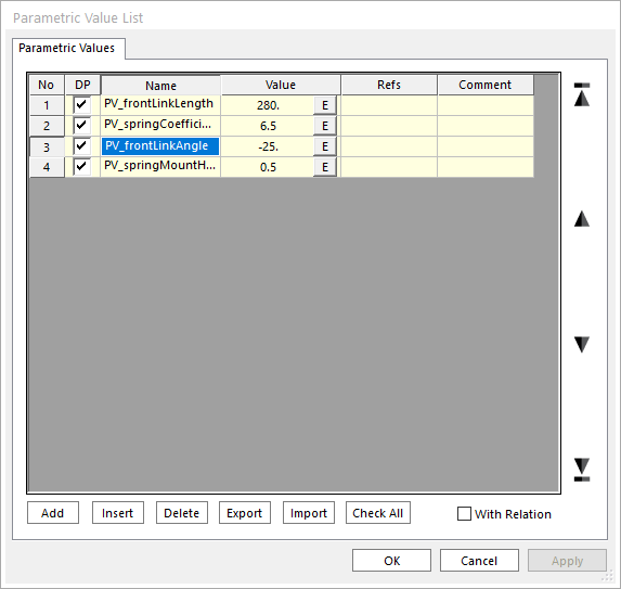
1. In the Database window, double-click on one of the items under Parametric Values shown in Figure 3.39.

   

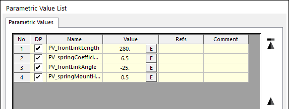
   Figure 3.39 Parametric Value List

2. Click or double-click on the value next to PV_frontLinkAngle and change it to -40.

3. Click OK, and then you can see how this change affects the catapult’s physical configuration.

4. Click Dynamic/Kinematic.

5. Click Simulate.

6. When the simulation stops, click Play and view the results.

7. Repeat the above steps, using different combinations of values for PV_frontLinkAngle and PV_springMountHeight, within the following ranges:

   • -40 ≤ PV_frontLinkAngle ≤ -10

   • 0.4 ≤ PV_springMountHeight ≤ 0.6

   If you do not wish to run through many simulations, Figure 3.40 ~ Figure 3.43 are several animation results representing the ends of the ranges for the two design variables.

   

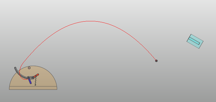
   Figure 3.40 1-2

   Analysis result that front link angle = -10 degree and spring mount height = 0.4

   

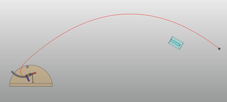
   Figure 3.41 1-3

   Analysis result that front link angle = -10 degree and spring mount height = 0.6

   

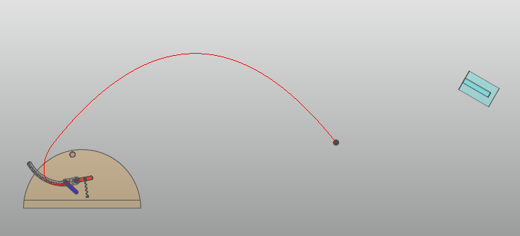
   Figure 3.42 1-4

   Analysis result that front link angle = -40 degree and spring mount height = 0.4

   

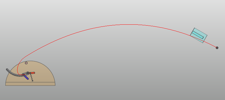
   Figure 3.43 1-5

   Analysis result that front link angle = -40 degree and spring mount height = 0.6

8. When you are finished exploring the model, return the parametric values to their original values before continuing with the tutorial (PV_frontLinkAngle = -25, PV_springMountHeight = 0.5).

3.2.4.2. Defining the Design Variables

3.2.4.2.1. To create a design parameter:

1. From the AutoDesign menu, click Design Parameter. This will bring up the Design Parameter List dialog shown below.

   

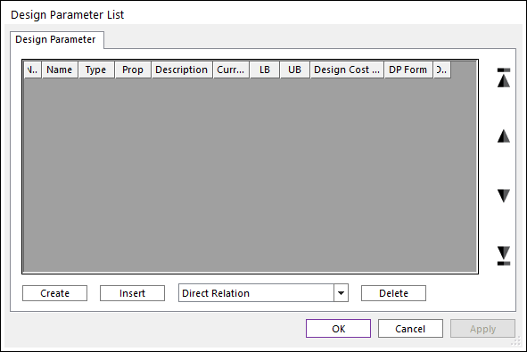
2. Click Create to create a new design parameter.

3. In the Direct Relation dialog that appears, change the name from DP1 to DP_frontLinkAngle.

4. Press Pv to bring up the Parametric Value List dialog. Select the PV_frontLinkAngle parametric value by clicking on its name. When selected, it should be highlighted in blue, as shown below.

   

5. Click OK to choose this as the design parameter.

6. Back in the Direct Relation dialog, define upper and lower bounds (-40, -10). Enter a description (Front link angle) in the Description field. When completed, the dialog should appear as shown at below.

   

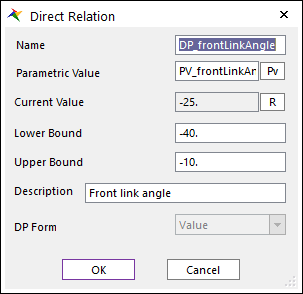
7. Press OK to return to the Design Parameter List dialog box.

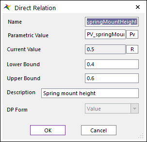
8. Create design parameter for spring mount height, similarly, using the following settings:

   • Name: DP_springMountHeight

   • Parametric Value: PV_springMountHeight

   • Lower Bound: 0.4

   • Upper Bound: 0.6

   • Description: Spring mount height

   

9. Return to the Design Parameter List dialog and check the checkboxes under the DV column for both of the design parameter you just created. This activates both as Design Variables, which will be used in the Design Study and Design Optimizations to follow. When completed, the Design Parameter List dialog should appear as shown below.

   

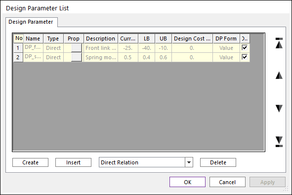
   Note

   To go back and edit a design parameter, click on the button under the Prop. column.

10. Press OK to close the Design Parameter List dialog box.

3.2.5. Defining the Performance Indexes

The performance indexes will tell you how well or poorly the model is able to perform its goal. In this case, these are the error of the ball’s angle of attack and how close it gets to the target. To obtain good optimization results, these goals are formulated as follows.

The position and velocity of the ball is measured with respect to the target’s reference frame. To evaluate the angular error of the ball, the ball’s velocity in the y-direction is measured as it crosses the target plane. A small y-directional velocity indicates a small angular error. To evaluate the positional error of the ball, the distance between the ball and the target is measured in the y-direction as the ball crosses the target plane, as shown in Figure 3.44.

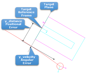
Figure 3.44 Performance indexes for design optimization

In addition, a third one is used, which is simply the measurement of the closest the ball ever comes to the target.

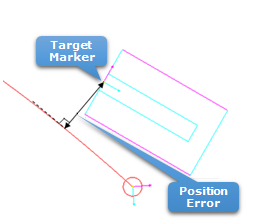
This formulation of the performance indexes may not be the most intuitive one, but it provides results which are the least sensitive to numerical noise.

3.2.5.1. To create an analysis response:

1. From the AutoDesign menu, click Analysis Response. This will bring up the Design Parameter List dialog shown below.

   

2. Click Create to create a new analysis response.

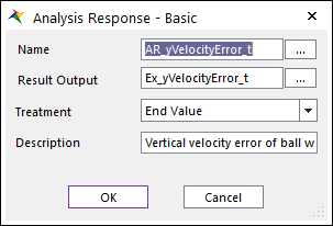
3. In the Analysis Response - Basic dialog that appears, change the name from AR1 to AR_yVelocityError_t.

4. Press EL to bring up the Expression List dialog. Select the Ex_yVelocityError_t expression by clicking on its name. When selected, it should be highlighted in blue as shown below.

   

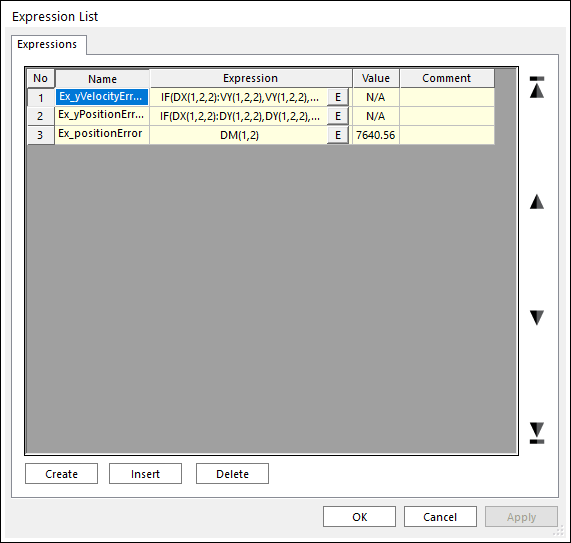
5. Click OK to choose this as the expression to use.

6. Back in the Analysis Response - Basic dialog, for the Treatment, select End Value from the dropdown list. Enter a description (Vertical velocity error of ball w.r.t. target.) in the Description field. When completed, the dialog should appear as shown at below.

   

7. Press OK.

   Note

   To go back and edit an analysis response, click the button under the Prop.Column.

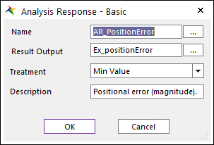
8. Create two more analysis responses using the following values:

   Name	AR_yPositionError_t	AR_positionError
   ResultOutput	Ex_yPositionError_t	Ex_positionError
   Treatment	End Value	Min Value
   Description	Vertical position error w.r.t. target.	Positional error (magnitude).

   The treatment parameter is used to control how you extract a single numerical value from a curve which varies over time. For example, setting the treatment to End Value will assign the value of the curve at the end of simulation, while Min Value will assign the lowest value that the curve reaches during the simulation.

   

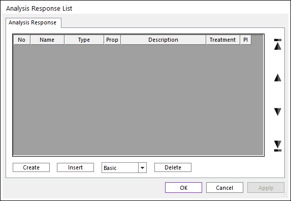
9. Return to the Analysis Response List window and check the checkbox under the PI column corresponding to the analysis responses you just created. This activates them as Performance Indexes, which will be used in the Design Study and Design Optimizations to follow. When completed, the Analysis Response List window should appear as shown in :Figure 3.45.

   

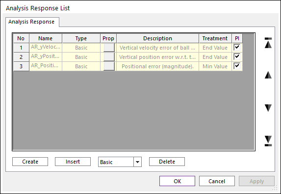
   Figure 3.45 Analysis response list

10. Press OK to close the Analysis Response List dialog.

11. Save the model.

3.2.6. Design Optimization

3.2.6.1. Objectives and Constraints

When performing optimizations, you can define objectives and constraints that will guide the optimization to the desired solution. Objectives are used when you want to minimize or maximize performance indexes. Our model has three performance indexes, of which one will be minimized using an objective. For other models, it is possible to have multiple objectives, and have different weights assigned to each one to specify how important it is relative to the other objectives. Constraints, on the other hand, are used when a specific requirement must be met in order for a solution to be considered successful.

For this problem, we may specify that the y-velocity error is less than 5(mm/sec), or that the y-position error must be less than 5(mm). From the viewpoint of ideal solution, these values should be equal to ‘0.0’. However, the numerical analysis cannot give those accurate results. Thus, the values of these limitations fully depend on the accuracy of numerical solvers.

3.2.6.2. AutoDesign’s Design Optimization Process

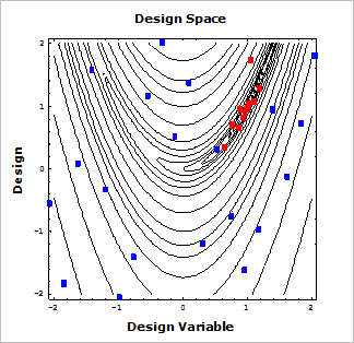
When AutoDesign performs an optimization, it first performs a design of experiment (DOE). During this process, it samples the design space at several points, evaluating the performance Design indexes given various combinations of the design variables. These points are indicated by the blue squares in the figure at below.

Next, AutoDesign fits an analytical surface to the points, called a meta-model. Using this meta-model, AutoDesign then determines the best point in the design space to search for the optimal solution. Then, evaluate the exact analysis for the selected optimum point. If this new design cannot satisfy the convergence criterion, then, the analysis results and design point are added to the original DOE tables and re-construct the meta-model. Then, the optimizer solves the optimization problem made from new-meta model. This process is repeated until all convergence criteria are satisfied. The red squares, shown in the figure, are the optimum points selected by optimizer. We call this optimization process as Sequential Approximate Optimization with Meta-Models (SAOM). For more information on the sampling algorithm, please refer to the AutoDesign Theoretical Manual.

3.2.6.3. Running a Design Optimization

We will now run an optimization in which the objective is to minimize the position error, and constraints are set on the y-velocity and y-position error.

3.2.6.3.1. To run a design optimization:

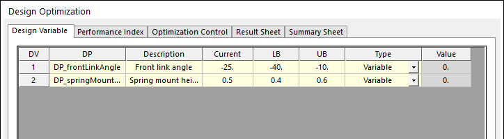
1. From the AutoDesign menu, select Design Optimization. The Design Variable dialog box should appear as shown below, by default.

   

2. Click on the Performance Index tab.

3. Change the objective function according to the table below.

   Performance Index	Definition	Goal	Weight/Limit Value
   AR_yVelocityError_t	Constraint	EQ	0
   AR_yPositionError_t	Constraint	EQ	0
   AR_positionError	Objective	MIN	1

   After making the changes, the dialog should appear as shown below.

   

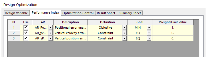
   Here, we are defining that the target values for the errors are 0, and at the same time we want to minimize the position error.

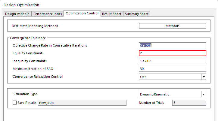
4. Click on the Optimization Control page.

5. Change the settings so that they appear as shown at below. As explained in the introduce of the Chapter 4, we will try to satisfy AR1 and AR2 .LE. 2. To do this, we define them as Equality Constraints and set their convergence tolerances to 2.0. This limitation fully depends on the resolution of dynamic analysis results.

   

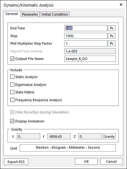
6. Check the analysis setting by clicking Analysis Setting. In order to reduce the numerical error, we increase the number of time steps shown in below. If you increase the resolution of optimization solution, then increase the number of steps. In refining the design optimization, we will show more accurate design by only increasing the value.

   

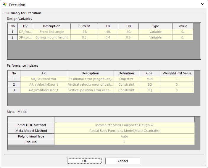
7. Click Execution to run the optimization with the settings you just made. Then, you can see the summary of the optimization formulation shown as below. Then, click OK. The optimization will be progressed.

   

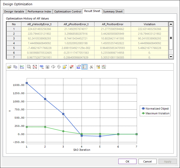
8. To view the result of the design optimization after optimization is completed, click the Result Sheet tab. The Performance indexes for optimization iterations are listed at the top of the dialog. To see the final result of the optimization shown as below, scroll down to the last iteration. As shown below, the final vertical velocity error is -1.34(mm/sec), and the final vertical position error is 0.053(mm). Also, the final position error is 6.19(mm). The optimization took 11 iterations to converge to these results.

   

9. To see the summary sheet, this shows the final values of design variables and analysis results. In the summary of SAOs, the total number of analysis, including the initial DOE, is 16.

3.2.7. Animating the Optimized Model

To animate the optimized model, we will first have to update the model with the optimized design variables.

3.2.7.1. To update the model with the optimized design variables:

1. From the AutoDesign menu, select Summary Sheet. The summary sheet is shown as the figure below.

   

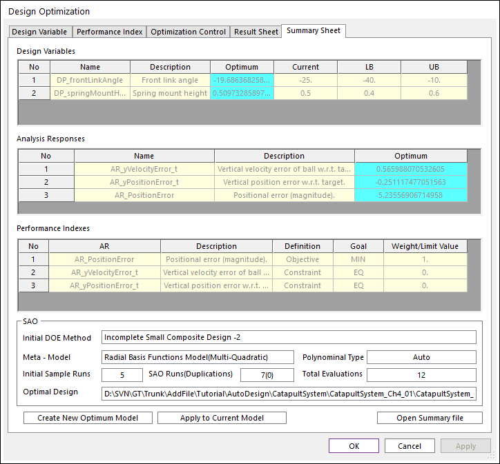
2. Check the box Create new Optimum Model, which is marked in the upper figure.

3. Then, enter the new file name as Sample_B_Opt.

4. Click Confirm.

   The model’s parametric values have now been updated. (This window can be brought up by selecting Parametric Value from the SubEntity.)

5. In the Database Window, under Contacts, right-click on GeoSurContact_ballToTarget and uncheck the Inactive option.

6. Click the Dynamic/Kinematic Analysis function on the Analysis tab.

7. Uncheck the checkbox next to Output File Name if it is checked.

8. Click Simulate. When the simulation is done, click Play. The ball should successfully make it into the target, as shown below.

   

   Before continuing with the tutorial, the model needs to be reset for the next optimizations.

3.2.7.2. To reset the model for the next optimizations:

1. Inactivate the contact between the ball and target.

2. Change the parametric values back to the initial values:

   • PV_frontLinkAngle = -25

   • PV_springMountHeight = 0.5

3. Save the model.