7.5. RFlexGen Crankshaft Tutorial (RFlexGen)
7.5.1. Overview
RecurDyn allows you to use FFlex and RFlex bodies to simulate flexible bodies in multi-body dynamic models. To create FFlex bodies in RecurDyn, you can simply apply the FFlex/Mesher to the rigid bodies that you want to make flexible. However, creating RFlex bodies in versions up to RecurDyn V8R2 required separate finite element (FE) software with an Eigen solver. So, you had to create files using the Eigen solver in the FE software and then process the files in RecurDyn to generate the RFlex bodies.
In this tutorial, we will show you the benefits of RecurDyn’s new function, RFlexGen, and how to use it to create an RFlex body in a multi-body dynamic model. The model we will use in this tutorial is an in-line 4-cylinder internal combustion engine that simulates the combustion processes that normally occur in an engine. We will achieve the objectives of this tutorial by examining the analysis outcomes when the crankshaft body is replaced by an FFlex or RFlex body.
7.5.1.1. Tutorial Objectives
In this tutorial, you will learn how to:
Create FFlex bodies using RecurDyn Mesher
Examine the dynamic characteristics of flexible bodies made using RecurDyn/FFlex
Create RFI files from FFlex bodies using RecurDyn/RFlexGen
Replace RFlex bodies using RecurDyn/RFlex and examine their dynamic characteristics
Create RFI files from RFlex bodies using RecurDyn/RFlexGen
Compare the dynamic characteristics of FFlex bodies and RFlex bodies
Recognize the benefits of using the RFlexGen function
7.5.1.2. Prerequisites
This tutorial is intended for users who have completed the Basic and FFlex/RFlex tutorials provided with RecurDyn. If you have not completed these tutorials, then we recommend completing them before proceeding with this tutorial. In addition, this tutorial requires a basic understanding of dynamics and the finite element method.
7.5.1.3. Tasks
The following table outlines the tasks involved in this tutorial and their duration.
Procedures |
Time (minutes) |
Opening the RecurDyn model |
10 |
Generating the FFlex body using the Mesher |
15 |
Analyzing the dynamic characteristics of the FFlex body |
10 |
Creating the RFI file using RFlexGen |
10 |
Replacing the existing body with the RFlex body |
5 |
Analyzing the dynamic characteristics of the RFlex body |
5 |
Creating another RFI file using RFlexGen |
5 |
Analyzing the dynamic characteristics of the RFlex body |
5 |
Comparing the analysis results |
10 |
Total |
70 |
7.5.1.4. Estimated Time to Complete
70 minutes
7.5.2. Opening the Initial Model
7.5.2.1. Task Objectives
This chapter teaches you how to open the initial model, run a simulation, and observe how the 4-cylinder engine model operates.
7.5.2.2. Estimated Time to Complete
10 minutes
7.5.2.3. Opening the RecurDyn Model
7.5.2.3.1. To run RecurDyn and open the initial model:
On your Desktop, double-click the RecurDyn shortcut. When the Start RecurDyn dialog box appears, close it.
In the File menu, click the Open function.
- Navigate to the RFlexGen tutorial folder, and then select RD_RFlexGen_4Cyl_Engine_Start.rdyn.(The file path: <InstallDir>\Help\Tutorial\Flexible\RFlexGen)
Click Open. The model shown below opens.
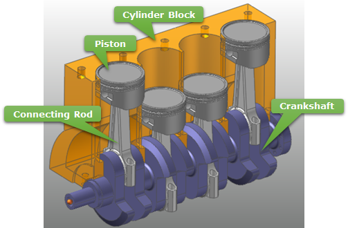
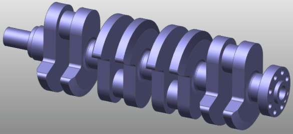
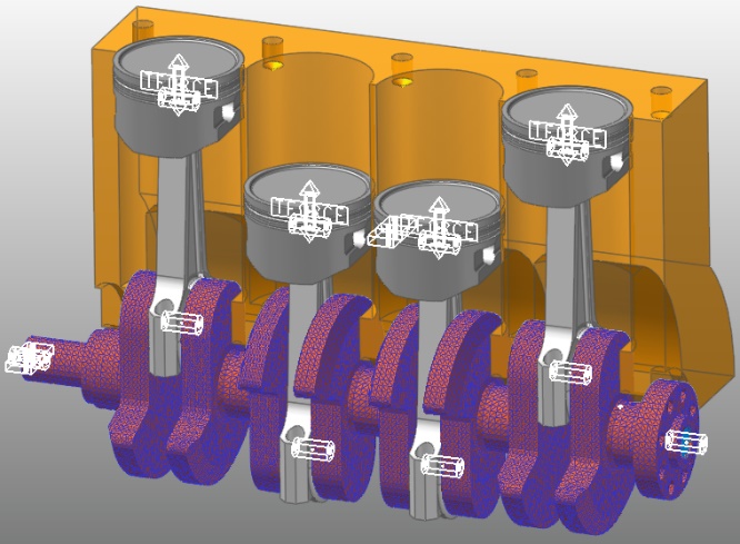
The configuration of the model is as follows.
The model is 4-cylinder in-line engine. It consists of a cylinder block, pistons, connecting rods, and a crankshaft. In an actual engine, the explosive force generated in the cylinder drives the pistons downward in the cylinder block. This causes the connecting rods attached to the pistons to rotate the crankshaft. To simulate this process in RecurDyn, the force generated by the explosion in the cylinder is converted into a force profile that applies force to each piston at the correct time.
7.5.2.3.2. To save the initial model:
- From the File menu, click the Save As function.(Save this model in the different path because it is impossible to simulate directly in the tutorial path.)
7.5.2.4. Running the Initial Simulation on the 4-Cylinder Engine Model
To understand the behavior of the model, we will perform an initial simulation using the model.
7.5.2.4.1. To perform the initial simulation:
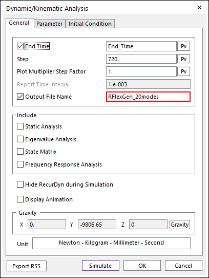
On the Analysis tab, in the Simulation Type group, click the Dynamic / Kinematic Analysis function. The Dynamic/Kinematic Analysis dialog box appears.
After verifying the simulation conditions, click Simulate.
7.5.2.4.2. To view the results:
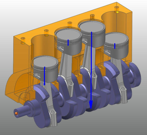
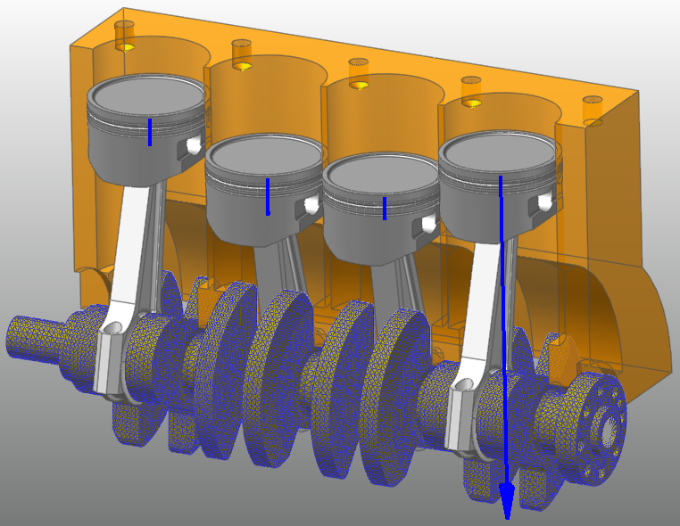
On the Analysis tab, in the Animation Control group, click the Play function to run the simulation.
If you look closely at the behavior of the model, you can see that the combustion occurs in the following order: Piston_1 -> Piston_3 -> Piston_4 -> Piston_2. This behavior is represented by the lengthening of the arrows, which represent the force in the animation. Although a typical four-cylinder engine’s stroke process consists of intake -> compression -> combustion -> exhaust, only the force generated by the combustion is meaningful in the dynamic model used for this tutorial. Therefore, the explosive force is converted into a force profile that applies force to each piston at the correct time.
7.5.3. Generating the FFlex Body
To analyze the multi-flexible body dynamics (MFBD) of the engine model, you must convert the crankshaft into a flexible body (FFlex body). This procedure maintains most of existing elements from the previous model, such as the joints and force. However, we will replace the rigid crankshaft with a flexible body to improve efficiency.
7.5.3.1. Task Objectives
This chapter teaches you how to replace an existing rigid body with a flexible body using the Mesher provided in RecurDyn FFlex (Full Flex).
7.5.3.2. Estimated Time to Complete
15 minutes
7.5.3.3. Creating the Crankshaft Mesh
7.5.3.3.1. To create the crankshaft mesh:
In Assembly mode, select the Crankshaft Body.
Right-click the screen to display the context menu, and then click Mesh.
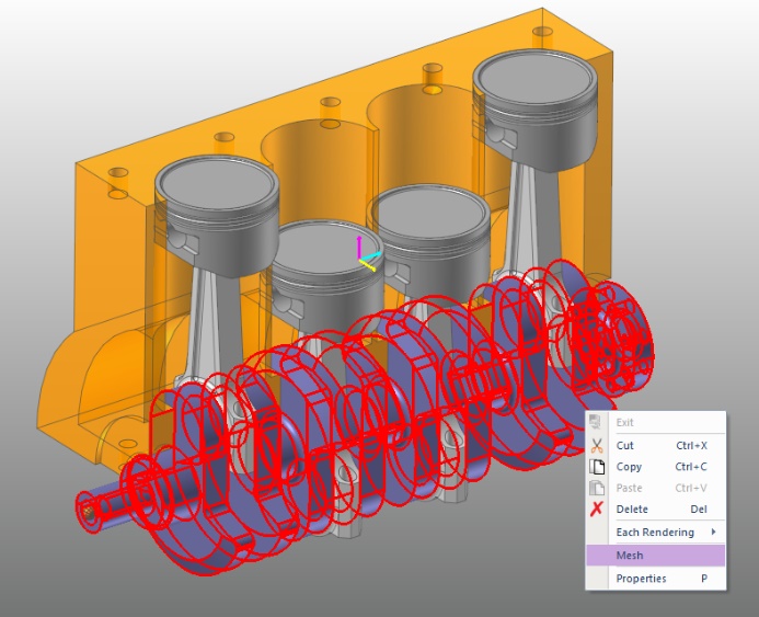
As shown below, Mesh mode only displays the crankshaft body.
On the Mesher tab, in the Mesher group, click the Assist Modeling function. The Assist Modeling dialog box appears.
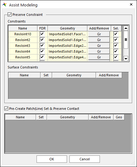
- Select the Preserve Constraint option.The joints connected to the crankshaft body appear in the Assist Modeling dialog box, as shown in the image to the below.
Tip
The Geometries in the Preserve Constraint are applied to the Assist Modeling dialog automatically after the user selects the Target Body. However, following behind steps are recommended to the user to produce accurate results, especially in the tutorial.
- In the Assist Modeling dialog box, select all the checkboxes in the FDR and Sel. columns.The checkboxes in the FDR column specify whether to generate FDR (Force Distributed Rigid) elements after creating the mesh. The checkboxes in the Sel. column specify whether to maintain the previous joints and forces. For this tutorial, you must select all the checkboxes.
Tip
If you have difficulty selecting entities, use the Select List function of the right-click popup menu to select it.
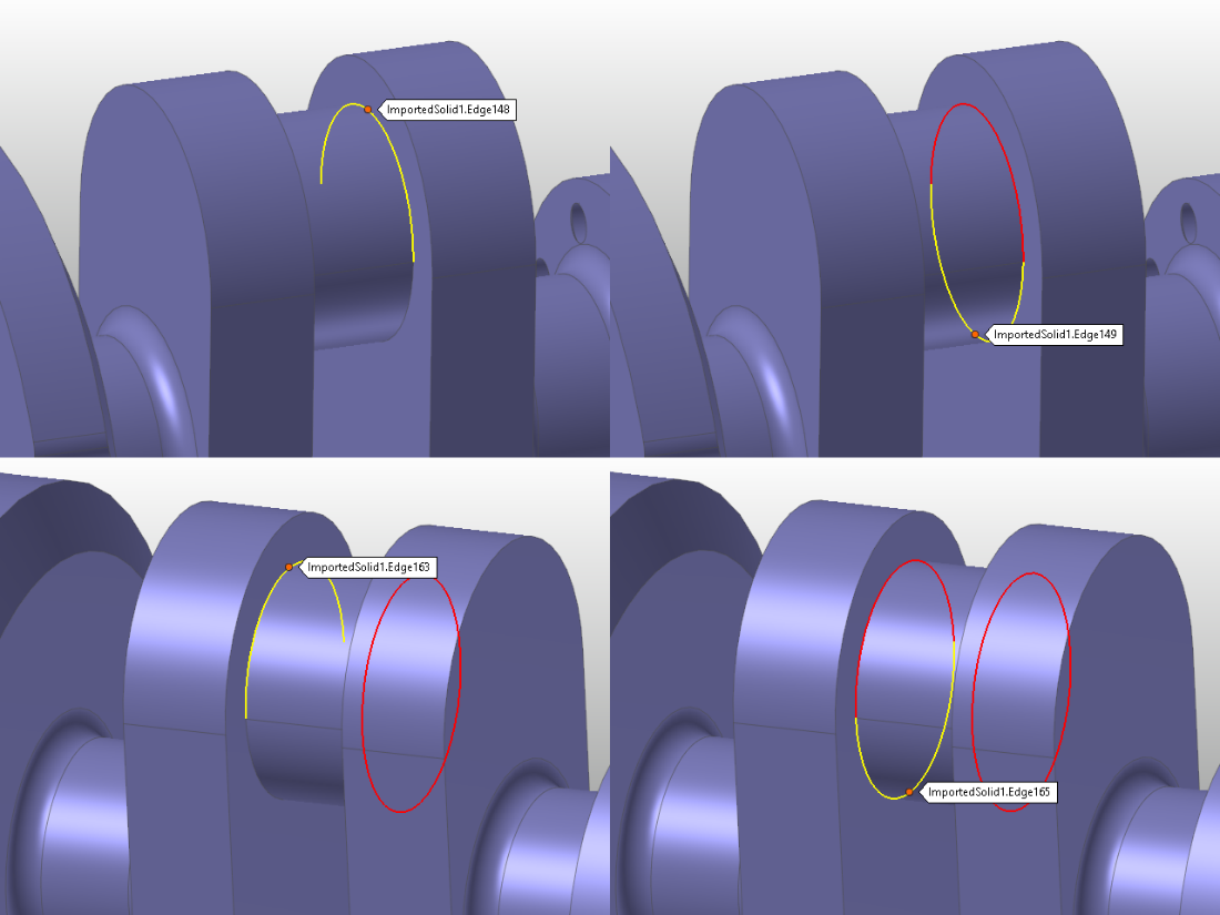
- In the Assist Modeling dialog box, in the Add/Remove column to the right of RevJoint2, click the Gr button. Then, click the appropriate geometries around RevJoint2 to set them as slave nodes.The edges around the master node will become the slave nodes for RevJoint2.
Select all four edges of the RevJoint2 master node. Then, right-click the node and click Finish Operation in the context menu.
Tip
Clicking Gr displays the markers for the master node. By using one, you can see the areas where the slave nodes should be created easily.
Tip
To display the tooltip for the selected edge at the correct location, as shown above, click the Snap to Grid tool in Select Toolbar.
Repeat the procedure described above to create slave nodes for RevJoint3, RevJoint4, and RevJoint5. However, RevJoint10 and Rev_Crankshaft only require you to select the two surfaces shown below.
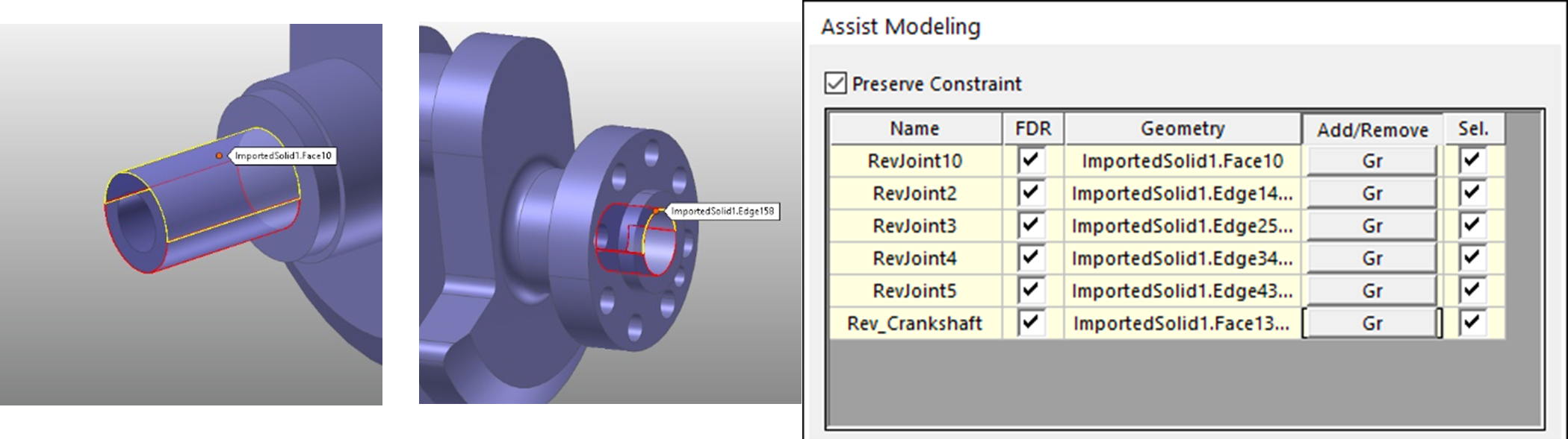
Confirm that the correct edges are selected for each geometry item, and then click OK.
On the Mesher tab, in the Mesher group, click the Advanced Mesh function. The Advanced Mesh dialog box appears.
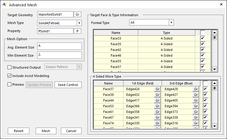
In the Advanced Mesh dialog box, perform the following steps:
In the Mesh Type dropdown menu, select Solid4(Tetra4).
In the Mesh Option group, set the Avg. Element Size to 4 and the Min Element Size to 2.
To change all of the faces in the 4 Side More Type list to 4 Side Type, select the checkbox to the right of the 3rd Edge heading.
Select the Include Assist Modeling option.
Tip
You must select this option to generate FDR elements automatically according to the conditions specified in the Assist Modeling dialog box.
Click Mesh.
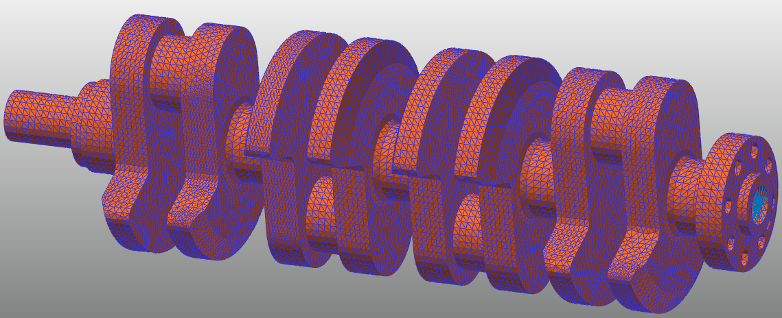
After the meshing process is complete, click Cancel.
The mesh model for the crankshaft body is generated, as shown below.
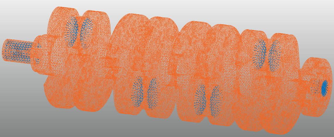
To see information about the FDR elements generated using the Assist Modeling function, change the view mode to Wireframe. Then, in the Database Window, under Property Components, select PFDR_1 to see all the FDRs generated for the crankshaft, as shown below.
Tip
RecurDyn Mesh mode includes two auto-meshers: Mesh and Advanced Mesh. Mesh applies tessellation to the geometry in the GUI before generating the mesh. Advanced Mesh skips the tessellation stage altogether and generates the mesh directly. By doing so, Advanced Mesh minimizes the distortion of the CAD geometry. However, Advanced Mesh also increases the failure rate when generating the mesh.To improve the mesh quality when using Advanced Mesh, change the faces in the 4-Side More Type list to 4-Side Type, as described above.To see the stress results for a specific node in the crankshaft as a plot, click the Output function in the FFlex Edit group, on the Mesher tab.
In the Output dialog box, perform the following steps:
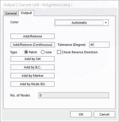
Click Add/Remove.
In the Input Window Toolbar, type 438 (node number), and then press Enter.

Right-click the Working window to display the context menu, and then click Finish Operation.
In the Output dialog box, click OK to create Output1 in the Database Window.
Perform either of the following steps to return to the parent mode:
Right-click the Working window, and from the menu that appears, click Exit.
From the Mesher group in the Mesher tab, click the Exit function.
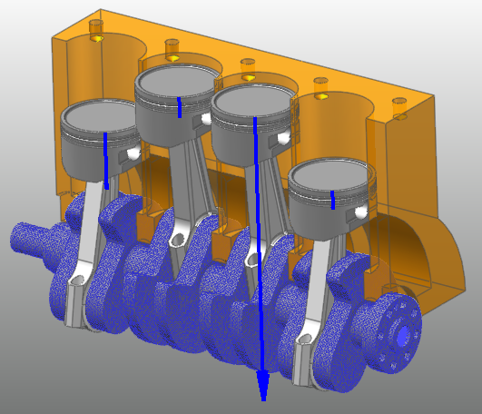
The existing crankshaft rigid body is replaced by the crankshaft flexible body (Crankshaft), as in the image below. However, the previous joints and forces remain the same. To see the icons, click the Icon Control tool in Render Toolbar to select all of the icons in the Working Window. (Click All Icons)
7.5.3.4. Conducting the Dynamic Analysis on the FFlex Body and Reviewing the Results
7.5.3.4.1. To conduct the dynamic analysis on the FFlex body:
Save the model as RD_RFlexGen_4Cyl_Engine_FFlex.rdyn.
Select Crankshaft, right-click the screen to open the context menu, and then click Properties. The Properties of Crankshaft dialog box appears.
In the dialog box, on the Body page, click Initial Velocity.
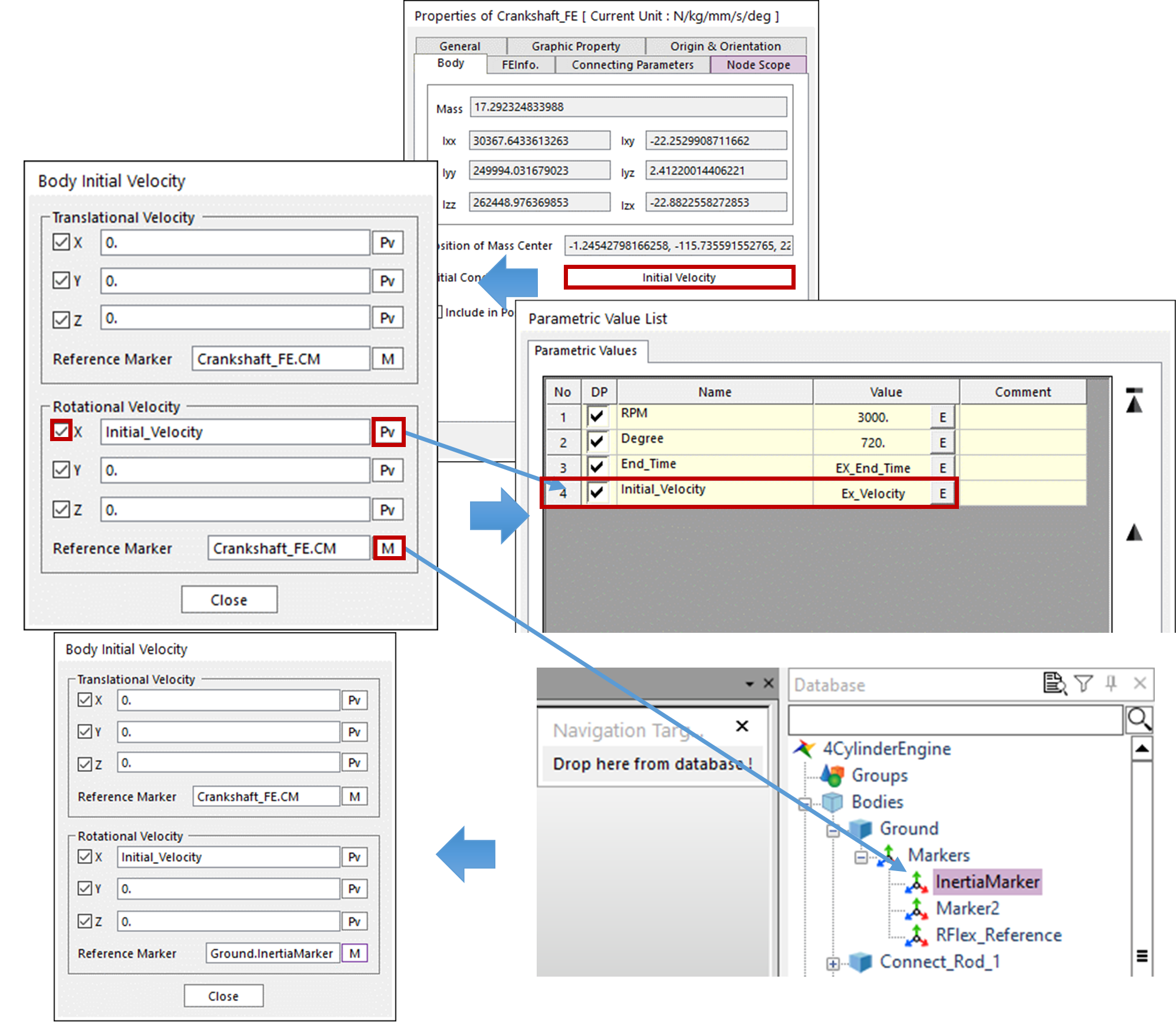
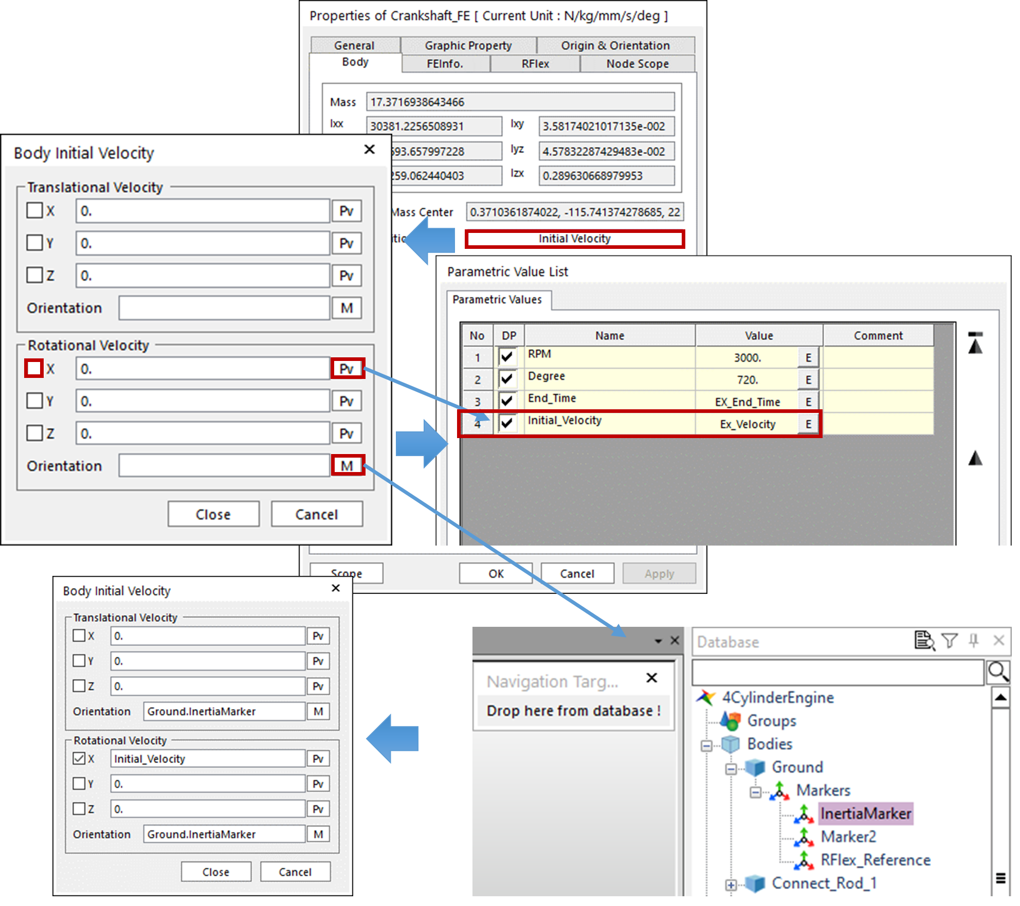
In the Body Initial Velocity dialog box, perform the following steps:
Select X in the Rotational Velocity group, and then click the PV button.
Select Initial_Velocity.
In the Reference Marker field, click the M button.
In the Database Window, under Ground, click the Inertia Marker and drag it to the Navigation Target window. Click Close to close the dialog window.
The following figure shows the entire process.
In the Properties of Crankshaft dialog box, on the Connecting Parameters page, clear the Use Force Connector checkbox.
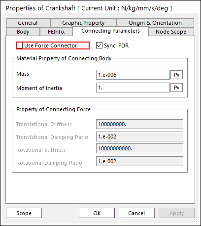
Click OK to close the dialog box.
Tip
If joints and forces are connected to a flexible body, then the RecurDyn Solver applies dummy bodies to the markers for the joints and/or forces to improve the efficiency of the calculation. That is, dummy bodies are connected to the flexible body using arbitrary high-strength force elements. In this tutorial, however, we bind the joints completely without using force elements to minimize the effects of the force at the joints where the connecting rods, which are rigid bodies, connect to the crankshaft, which is a flexible body. Also, although FDR elements can be divided into force elements and constraint elements, we exclude the force elements in this tutorial. This allows us to simulate the behavior of the flexible body more realistically, but it takes more time to analyze the model.
On the Analysis tab, click the Dynamic / Kinematic Analysis.
- In the Dynamic/Kinematic Analysis dialog box, click Simulate to run the analysis without changing any settings.The analysis duration may differ depending on the specifications of your PC, but it generally takes about an hour. Once the analysis is finished, play the animation. The animation should show results that are very similar to those obtained when the crankshaft is a rigid body.
If you only want to learn how to use RFlexGen, you may skip the rest of this chapter and proceed directly to chapter 4.
On the FFlex tab, click the Contour function.
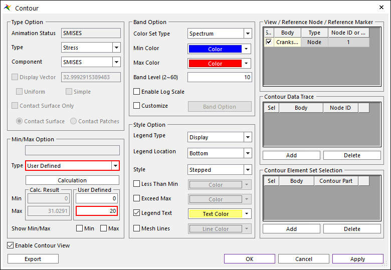
When the Contour dialog box appears, perform the following steps:
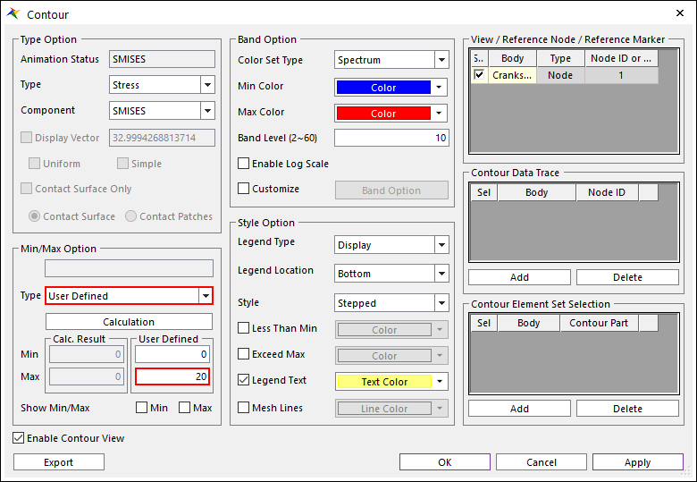
In the Min/Max Option group, click Calculation.
In the Min/Max Option group, set the Type to User Defined.
In the Max value text box, type 20.
Click OK to close the dialog box.
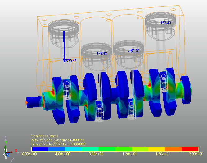
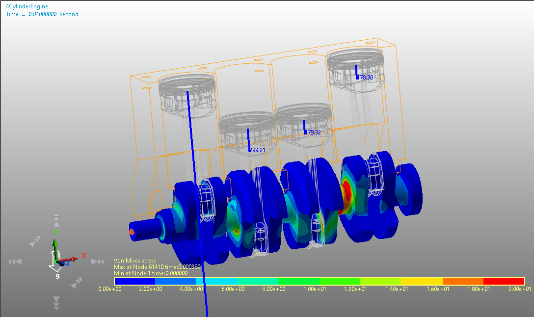
Click the Play function. The results should resemble those shown in the image to the below.
7.5.4. Generating the RFlex Body Using RFlexGen
7.5.4.1. Task Objectives
In this chapter, you will learn how to transform the FFlex body into an RFlex body using RFlexGen.
7.5.4.2. Estimated Time to Complete
40 minutes
7.5.4.3. Running RFlexGen
7.5.4.3.1. To run RFlexGen:
On the Flexible tab, in the Flex Interface group, click the RFlexGen function.
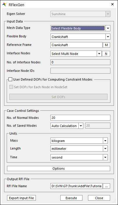
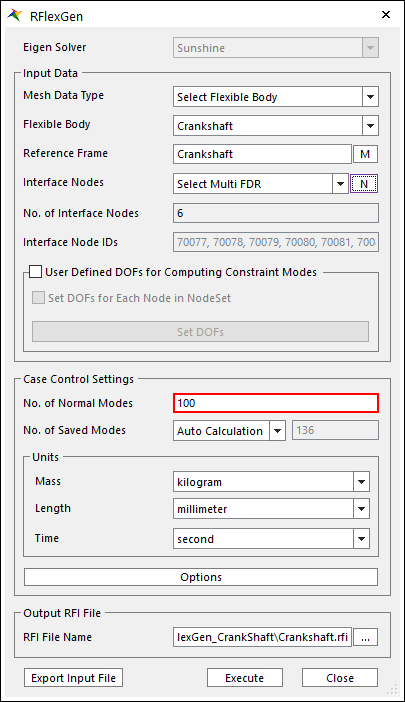
In this tutorial, Crankshaft is the only FFlex body. Therefore, the FFlex Body and Reference Frame fields are automatically filled, as shown in the figure above.
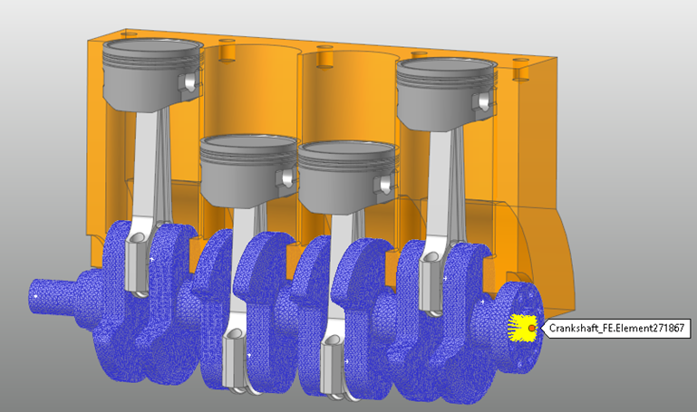
In the Interface Nodes dropdown menu, select Select Multi FDR. Then, click N and select FDR elements with dragging the mouse on Working Window.
Click Finish Operation on a mouse Right Menu. that was created earlier by selecting the master nodes in the Working Window.
In the RFlexGen dialog box, set the following options:
In the Case Control Settings group, set the No. of Normal Modes to 20.
In the Units group, maintain the default settings.
You do not need to change the units if the FFlex body was generated using RecurDyn/Mesher.
Click …, and then specify the name and folder path of the RFI file to create.
When you specify the path of the file, be sure to include the file name as well.
Ensure that the settings match those in the figure to the below.
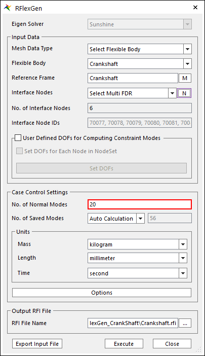
After adjusting the settings, click Execute.
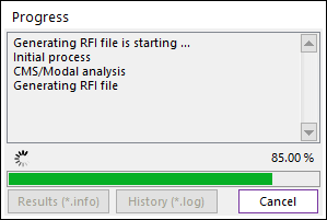
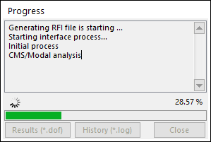
Wait as the Eigen solver performs the component mode synthesis (CMS) analysis.
Tip
Click the History (*.log) button to see details about the CMS analysis. If a problem occurs during the analysis, check the log file. Click the Results (*.dof) button to see the Eigen values for each mode after the analysis.
Once the analysis is complete, click Close to exit the RFlexGen progress window.
7.5.4.4. Creating the RFlex Body
7.5.4.4.1. To create the RFlex body:
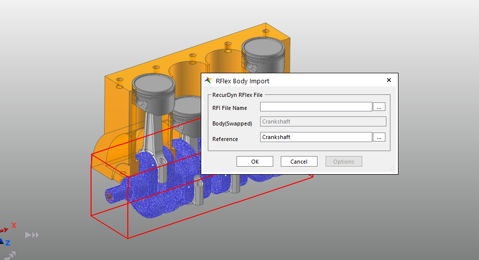
On the Flexible tab, in the RFlex group, click the Import RFI function.
Change the modeling option to Body.
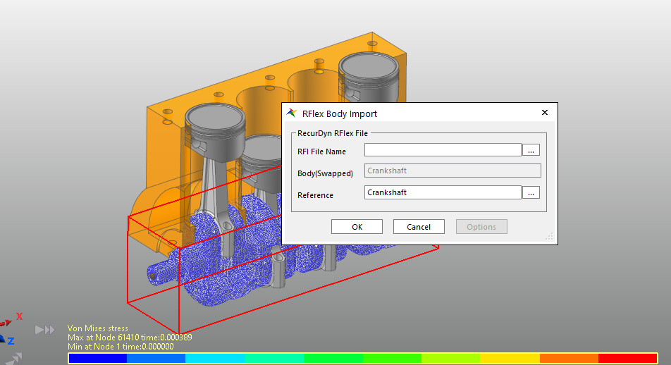
In the Working Window, select Crankshaft, as shown below. The RFlex Body Import dialog box appears.
In the RFlex Body Import dialog box, perform the following:
Click … to the right of the RFI File Name field.
Select the RFI file that you created in the Running RFlexGen chapter.
Click … to the right of the Reference field, and then select Crankshaft. (Ensure that the Reference field displays Crankshaft.)
Tip
You can use the name of FFlex body or RFlex body in the Reference field to automatically set the Body Reference Frame of the flexible body. Therefore, the above procedure sets the Body Reference Frame of the crankshaft FFlex body to the reference frame of the Flex body instead of the center marker (CM) of the body.
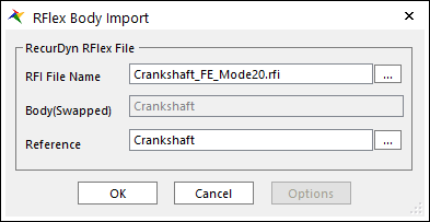
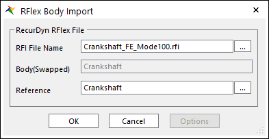
Ensure that the selected conditions match those shown in the figure to the below, and then click OK.
Click the Icon Control tool in Render Toolbar.
In the Icon Control dialog box, select All Icons.
In the Working Window, ensure that all of the joints that were applied to the crankshaft are still applied to RFlexBody1.
After verifying the joints, clear the checkboxes in the Icon Control dialog box.
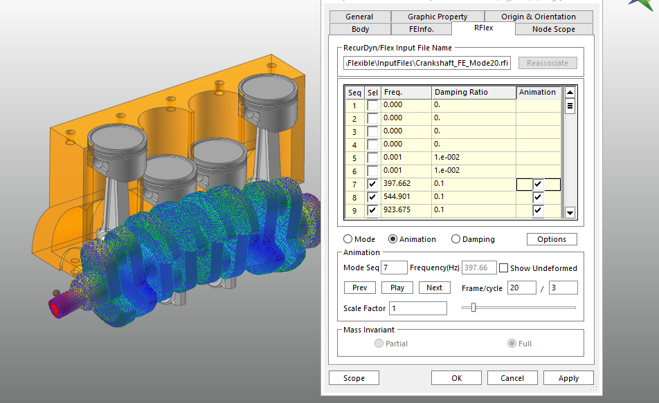
In the Database Window, double-click RFlex body to open the Properties dialog box.
In the Properties dialog box, perform the following:
Click 7th mode, as shown in the figure to the below.
Click Play to observe the behavior of the selected mode. The animation shown in the following figure appears so that you can observe the behavior of the mode.
You can also observe the model in other modes by performing the above steps and changing the mode.
7.5.4.5. Conducting a Dynamic Analysis on the RFlex Body and Reviewing the Results
7.5.4.5.1. To conduct a dynamic analysis on the RFlex body:
Select RFlexBody1, right-click it to display the context menu, and then click Properties. The Properties of RFlexBody1 dialog box appears.
In the Properties of RFlexBody1 dialog box, on the Body page, click Initial Velocity.
In the Body Initial Velocity dialog box, perform the following steps:
Select X in the Rotational Velocity group, and then click Pv.
Select Initial_Velocity.
In the Reference Marker field, click M.
In the Database Window, under Ground, click the Inertia Marker and drag it to the Navigation Target window. Click Close to close the dialog window.
The following figure shows the entire process.
In the Database Window, double-click RFlexBody1 to enter RFlex Edit mode.
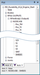
To see the stress result for a specific node in RFlexBody1 as a plot, click Output in the RFlex Edit menu.
In the Output dialog window, perform the following steps:
Click Add/Remove.
In the input field of the Input Window Toolbar, type 438 (node number), and then press Enter.
Right-click the screen to display the context menu, and then click Finish Operation.
In the Output dialog box, click OK to create Output1 in the Database Window.
Right-click the screen to display the context menu, and then click Exit.
On the Analysis tab, click the Dynamic/Kinematic Analysis function to open the Dynamic/Kinematic Analysis dialog box.
In this Dynamic/Kinematic Analysis dialog box, set the Output File Name as RFlexGen_20modes. Click Simulate to run the analysis without changing any settings.
After about 10 seconds of analysis, you can see that the animation is similar to the previous crankshaft body animation. The analysis duration differs depending on whether you use an FFlex body or RFlex body. Therefore, we recommend performing the analysis with the body that best suits your purposes to improve efficiency.
On the Flexible tab, in the RFlex group, click the Contour function to open the Contour dialog box.
In the Contour dialog box, perform the following:
In the Min/Max option group, click Calculation.
In the Min/Max Option group, set the Type to User Defined.
In the Max value text box, type 20.
Click OK to close the dialog box.
Click the Play function. You should see the following results.
7.5.4.6. Running RFlexGen Again
7.5.4.6.1. To increase the number of modes and repeat the analysis, perform the following steps:
- On the Flexible tab, in the Flex Interface group, click the RFlexGen function.In the Generate RFI dialog box, you can see that Flexible Body and Reference Frame match the information for the previously created RFlex body, unlike when you opened the RFlexGen dialog box in the previous procedure.
In the Interface Nodes dropdown menu, select Select Multi FDR. Then, click N and select FDR elements with dragging the mouse on Working Window.
click Finish Operation on a mouse Right Menu. that was created earlier by selecting the master nodes in the Working Window.
In the RFlexGen dialog box, perform the following:
In the No. of Normal Modes field, type 100.
In the Units group, maintain the default settings.
In the Output RFI File group, click …, and then specify the name and folder path of the RFI file.
- After adjusting the settings, click Execute.The Eigen solver performs the CMS (component mode synthesis) analysis, as shown in the figure to the below.
Once the analysis is complete, click Close to stop the RFlexGen process.
7.5.4.7. Replacing an RFlex Body
7.5.4.7.1. To replace an RFlex body:
On the Flexible tab, in the RFlex group, click the Import RFI function.
Set the Creation Method to Body.
In the Working Window, select the Crankshaft, as shown below. The RFlex Body Import dialog box appears.
In the RFlex Body Import dialog box, perform the following:
Click … to the right of the RFI File Name field, and then specify the path and name of the RFI file (as described in the Running RFlexGen chapter).
Click … to the right of the Reference field, and then ensure that the name in the reference field has changed from Crankshaft.CM to Crankshaft.
Verify that the selected conditions match those shown in the figure to the below, and then click OK.
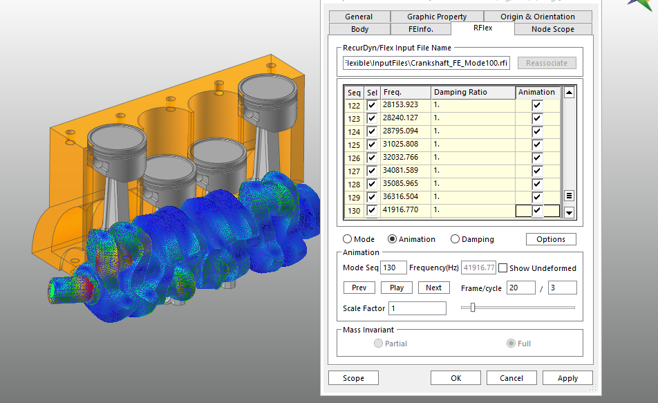
In the Database Window, double-click Crankshaft to display the Properties dialog box.
In the Properties dialog box, perform the following.
Select the 130th mode, as shown in the figure to the below.
Click Play to observe the behavior of the selected mode.
7.5.4.8. Conducting a Dynamic Analysis on the RFlex Body and Reviewing the Results
7.5.4.8.1. To conduct a dynamic analysis on the RFlex body:
7.5.5. Analyzing and Reviewing the Results
7.5.5.1. Task Objectives
In this chapter, we will analyze the results obtained from performing multi flexible body dynamics (MFBD) analyses on models containing FFlex or RFlex bodies and describe the benefits of using the RFlexGen function.
7.5.5.2. Estimated Time to Complete
5 minutes
7.5.5.3. Analyzing the Dynamic Analysis Results
7.5.5.3.1. Analysis of the results obtained from an FFlex body that was generated using the Mesher function
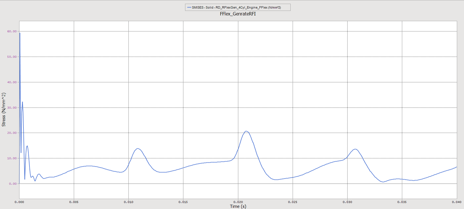
Earlier in this tutorial, we changed the crankshaft rigid body into a flexible body using the RecurDyn/Mesher and then performed a dynamic analysis. The flexible body included about 50,000 nodes (about 0.15 million degrees of freedom). Because of this, it took about 1 hour to perform the dynamic analysis. (The actual time may differ depending on the specifications of your PC.)
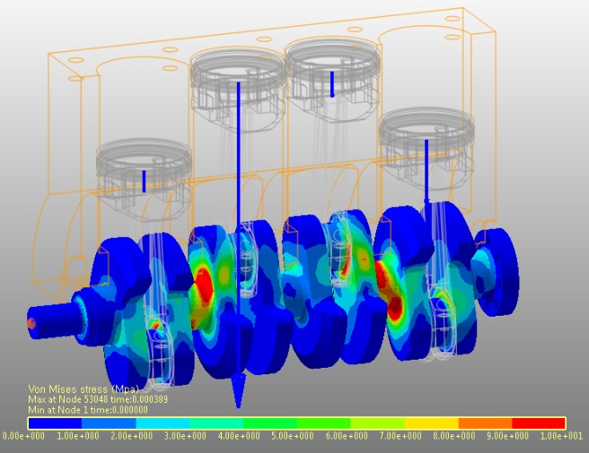
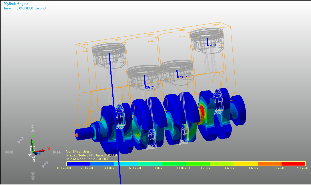
The following figure shows the results of the Von-Mises Stress test performed on the nodes that were included in the area of interest in the analysis results. (Since we defined the Output in the earlier steps, the test results were stored as a plot.)
7.5.5.3.2. Comparison of these results with the results obtained using an RFlex body that was generated using RFlexGen
The following figure compares the results of the Von-Mises Stress test using an FFlex body with those of an RFlex body. RFlexGen was used to transform the FFlex body into an RFlex body. The Von-Mises Stress test was performed on the nodes included in the area of interest in the analysis results.
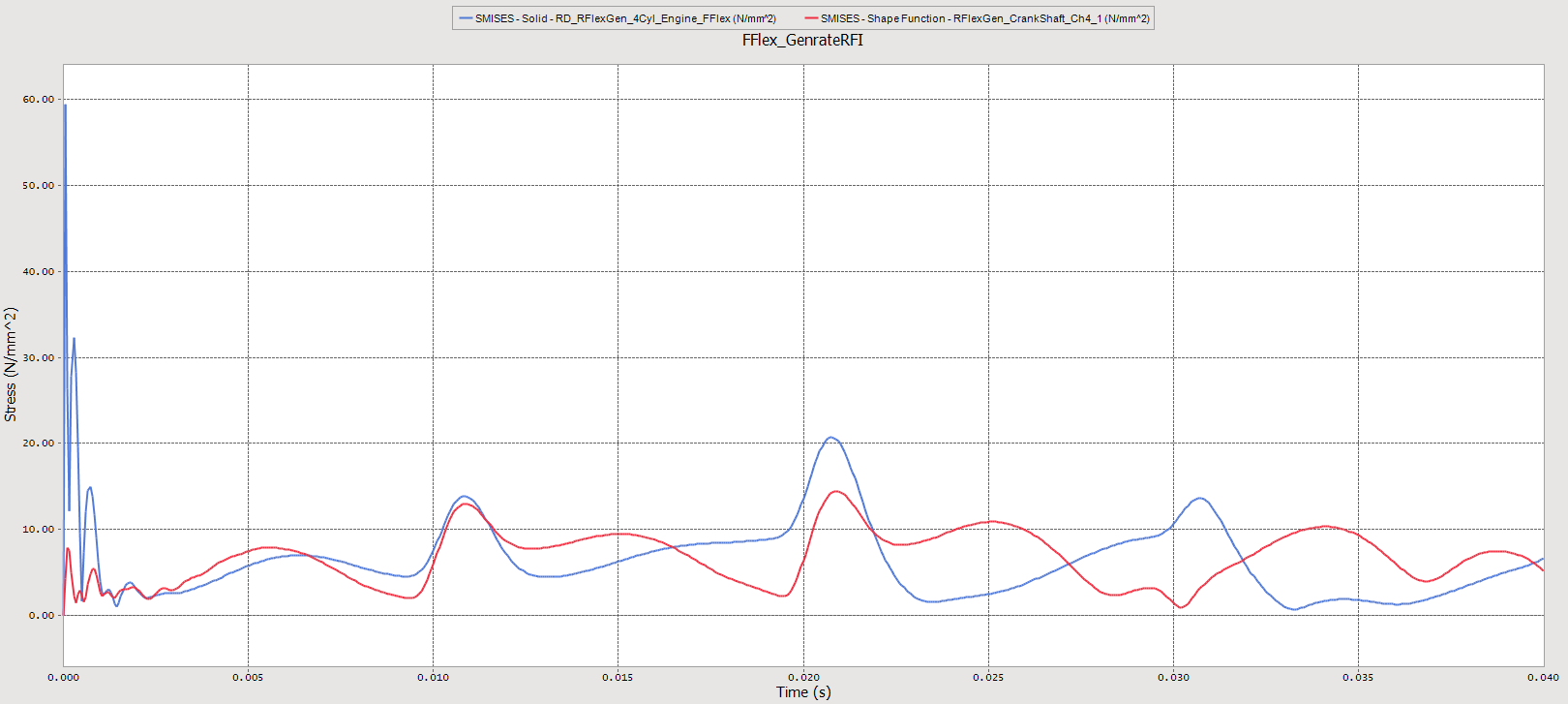
For the crankshaft used in this tutorial, we do not need to consider its contact with other bodies and the crankshaft is only bound by joints. Therefore, we don’t need an FFlex body to simulate the flexibility of the crankshaft because an RFlex body is sufficient for that purpose. That is, in an analysis situation that has many nodes for the flexible body and does not require any contact conditions, it is more efficient to use an RFlex body than an FFlex body if you require faster feedback more than accurate results.
As we can see in the above figure, there is not much difference between the results obtained with an FFlex body and the results obtained with an RFlex body. Considering the fact that the analysis using the RFlex body took only about 10 seconds while the analysis using the FFlex body took about 1 hour, you can see that using an RFlex body drastically reduces the time required for analysis while producing almost the same results as the FFlex body.
7.5.5.3.3. Comparison of the results after increasing the number of normal modes
The following figure shows the results after quintupling the number of normal modes for the RFlex body.
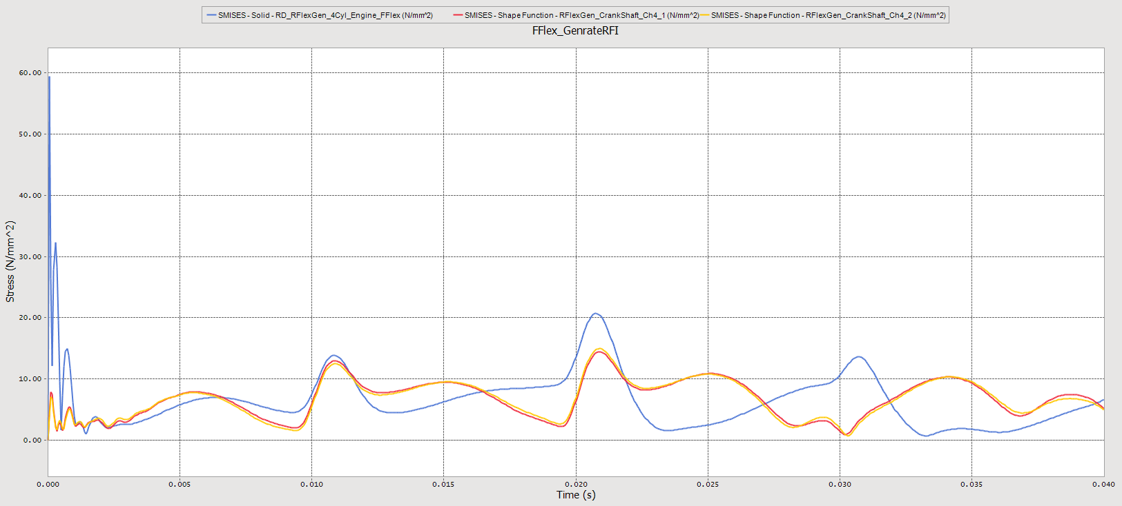
As you can see from the graph above, increasing the number of normal modes has little effect on the analysis results. From this, we can conclude that using a small number of normal modes in the engine system used for this tutorial still produces fairly accurate results.
7.5.5.3.4. Pros and cons of using an RFlex body generated by RFlexGen
This tutorial reveals the following pros and cons for using FFlex bodies and RFlex bodies.
Analyses using FFlex bodies produce more accurate results than those using RFlex bodies. This is because such analyses include the non-linear behavior of the analysis targets, including targets that have several contact conditions. In these cases, an FFlex body allows you to obtain more accurate results. However, the analysis takes longer if the number of nodes constituting the FFlex body or the number of non-linear properties of the target increases.
One benefit of using RFlex bodies is that they significantly reduce the analysis time. This is because the analysis uses the number of normal modes, instead of the number of total nodes, as the degree of freedom. Also, if the target behavior does not include non-linear properties that cause large scale transformations, then you can use an RFlex body to simulate the properties of a flexible body. However, in an MFBD model that requires an analysis of non-linear behavior, using an RFlex body instead of an FFlex body may reduce the accuracy of the analysis results. If you don’t need to simulate non-linear properties, then using an RFlex body can produce results much more quickly than using an FFlex body. This allows you to apply the analysis results in the design of the actual product much more quickly.