9.5. Piston Lubrication (EHD)
9.5.1. Overview
9.5.1.1. Task Objectives
The objective of fluid lubrication is to penetrate into the contact area between solid objects, which generate friction, and to form a thin oil film to reduce abrasion and frictional heat caused by friction. This oil film separates two solid surfaces from directly contacting each other and reduces friction and heat between them to smooth their movement.
The history of the lubrication theory started with an equation derived from the fluid flow existing in the narrow gap between two solid objects. The equation was presented by O. Reynolds back in 1886. This equation, called the Reynolds equation named after him, established the basis of the lubrication theory.
In this tutorial, EHD (elastic, hydraulic, and dynamic) elements, which are developed based on the Reynolds equation, are used to model the lubrication action at the part where the cylinder and the piston in the engine system contact each other and to perform the dynamic analysis of the cylinder and the piston considering their lubrication characteristics.
Configure the piston lubrication using the rigid model.
Swap the rigid bodies with the RFlex bodies, perform the analysis of the piston lubrication, and check the result of the lubrication action.
9.5.1.2. Prerequisites
This tutorial is intended for users who have completed the basic tutorials provided with RecurDyn. If you have not completed these tutorials, then you should complete them before proceeding with this tutorial.
9.5.1.3. Procedures
This tutorial consists of the following tasks and the time required for each task is listed in the table below.
Procedures |
Time (minutes) |
Opening the initial Model |
10 |
Analyzing Piston Lubrication with Rigid Bodies |
30 |
Analyzing Piston Lubrication with RFlex Bodies |
30 |
Analyzing the Results |
10 |
Modifying Piston Profile and Analyzing PistonLubrication |
10 |
Total |
90 |
9.5.1.4. Estimated Time to Complete this Task
90 minutes
9.5.2. Opening the Initial Model
9.5.2.1. Task Objectives
To open and observe the initial model.
9.5.2.2. Estimated Time to Complete This Task
10 minutes
9.5.2.3. Opening the RecurDyn Model
9.5.2.3.1. To run RecurDyn and open the initial model
On the Desktop, double-click the RecurDyn icon to open RecurDyn. When the Start RecurDyn dialog window appears, close it.
In the File menu, click the Open function.
- Navigate to the tutorial folder and select PistonLubricationEHD_Start.rdyn.(The file path: <InstallDir>\Help\Tutorial\Toolkit\EHD\PistonLubrication).
Click Open. to open the model shown in the following figure.
The following explains the configuration of the model.
An engine block consists of a cylinder, a piston, a piston pin, a connecting rod and a crank. The piston moves via the translation force defined with the spline of gas force according to the crank angle. The piston and the cylinder are joined by a translation joint, which makes the piston only move up and down.
9.5.2.3.2. To save the model:
- In the File menu, click the Save As function.(You cannot perform the simulation if the model is in the tutorial path, so you must save the model in a different path.)
9.5.2.4. Performing Simulation
This section teaches you how to perform an initial simulation using the model in order to understand its behavior.
9.5.2.4.1. To perform the initial simulation:
On the Analysis tab, in the Simulation Type group, click the Dynamic / Kinematic Analysis function.
The Dynamic/Kinematic Analysis dialog window appears.
After verifying the simulation conditions, click Simulate.
9.5.2.4.2. To view the result:
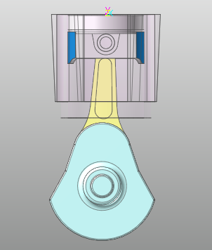
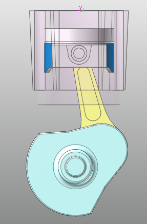
Under the Analysis tab, in the Animation Control group, press the Play function to check if the connecting rod moves as shown in the figure below.
9.5.3. Analyzing Piston Lubrication with Rigid Bodies
9.5.3.1. Task Objectives
For the lubrication analysis using EHD, you should define the cylinder and the piston of the engine system as the piston lubrication force. In this chapter, we will keep the modeling elements, such as joint and force, configured in the previously opened model as is, and define the piston lubrication to simulate and analyze the lubrication action of the rigid bodies.
9.5.3.2. Estimated Time to Complete This Task
30 minutes
9.5.3.3. Creating piston lubrication
From the previous model, delete TraJoint1 which was defined for movement.
Under the Toolkit tab, in the Toolkit group, click the Piston Lubrication function.
For the Creation Method, select Body, Point, Direction, Direction, Body, Point, Direction, Direction.
For the first body, select Cylinder, which is to be the Base Body, and click 0,-46.5,0, which is the middle part of the entire cylinder.
Use the Distance Measure function to check it.

Enter 0,1,0 for the axis on which the base body moves, and 1,0,0 for its direction of rotation.
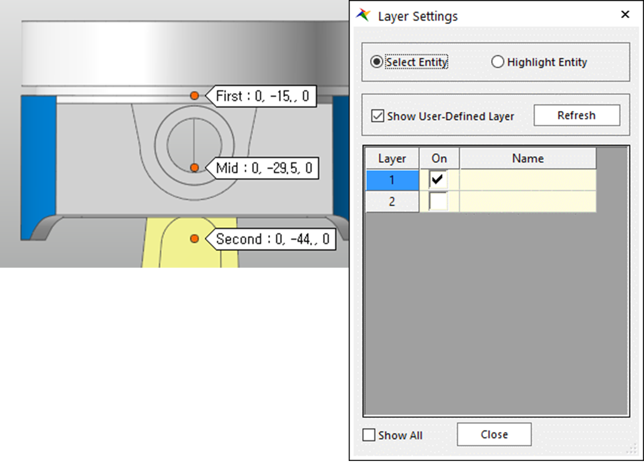
For the second body, select Piston, which is to be the Action Body, and click 0,-29.5,0, which is the middle part of the area contacting the cylinder.
From the Layer Settings window, uncheck Show All and uncheck the layer to which the cylinder body belongs so that you can select the piston body easily.
Enter 0,1,0 for the axis on which the action body moves, and 1,0,0 for its direction of rotation. You should set directions the same as those set for the cylinder body.
Make sure that the forces have been created in the Database Window.
9.5.3.4. Defining Piston Lubrication
In the piston lubrication created just before, we set the default values without considering the actual geometry of the cylinder and the piston. Now you should set them with the values of the geometry again.
Right-click Lubrication1 and select Properties in the context menu.
Enter 70 in the Piston Diameter field, 29 in the Piston Height field, 70.045 in the Cylinder Diameter field and 95 in the Cylinder Height field.
The value of the initial gap between the cylinder and the piston is the difference between both diameters divided by 2. In this tutorial, it is 0.0225.
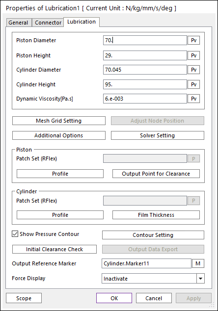
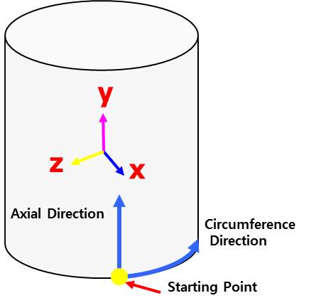
Click Mesh Grid Setting to adjust the mesh size. Enter 42 in the Circumference Node No. field and 21 in the Axial Node No. field.
For each direction, refer to the figure at the below.
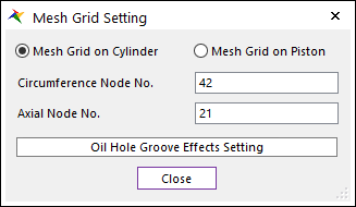
If the circumferential and axial directions have similar mesh grid sizes, you can perform the EHD analysis more efficiently.
In this tutorial, the sum of the circumferential length is \(70.075*pi = 220.05\) and its height is 95. Therefore, if you want to use the mesh grid of the size of about 5 mm, the appropriate quantity in the circumferential direction is 44 and that in the axial direction is 19.
For the asperity contact, click Additional Options to configure additional settings. If the thickness of the oil film becomes less than the roughness multiplied by 4 during the lubrication action, the asperity contact occurs.
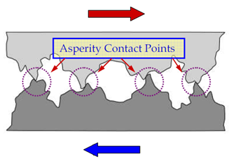
Enter values for the parameters to calculate the asperity contact as follows:
Roughness: 0.001
Composite Elastic modulus: 68000
Elastic Factor: 0.003
Friction Coefficient: 0.5
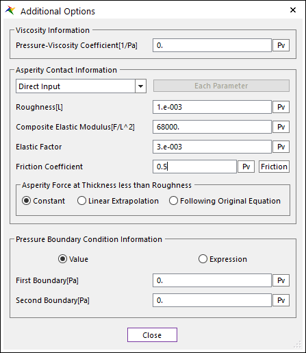
Click Close to close the window and click OK in the Properties dialog window for Lubrication1 to close it.
9.5.3.5. Performing Dynamic Analysis on Piston Lubrication and Checking Its Result
9.5.3.5.1. To run the simulation for piston lubrication:
Save the model as PistonLubricationEHD_Rigid.rdyn.
On the Analysis tab, in the Simulation Type group, click the Dynamic / Kinematic Analysis function.
The Dynamic/Kinematic Analysis dialog window appears.
After verifying the simulation conditions, click Simulate.
9.5.3.5.2. To view the result:
On the Analysis tab, in the Animation Control group, click the Play function to view the animation.
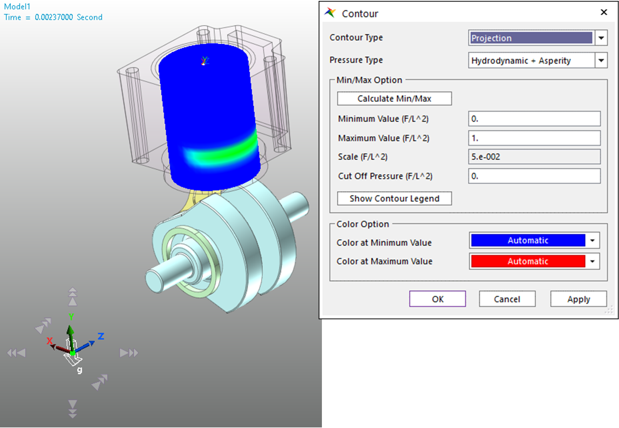
Right-click Lubrication1 and select Properties on the context menu.
Click Contour Setting and select Hydrodynamic + Asperity for Pressure Type.
You will be able to check the total lubrication force.
Change the Maximum Value field to 1 and click OK to close the window.
Play the animation again to see that the maximum values appear at both sides of the piston.
Click the Output Data Export button in the Properties dialog window for Lubrication1.
You can view the lubrication thickness and pressure from the top using a graph.
Select Thickness. In Angle base, enter 80 in the Frame for Plotting Time field and 4 in the Circum. Line field.
Click the View button to check Circumference Line and click Plot.
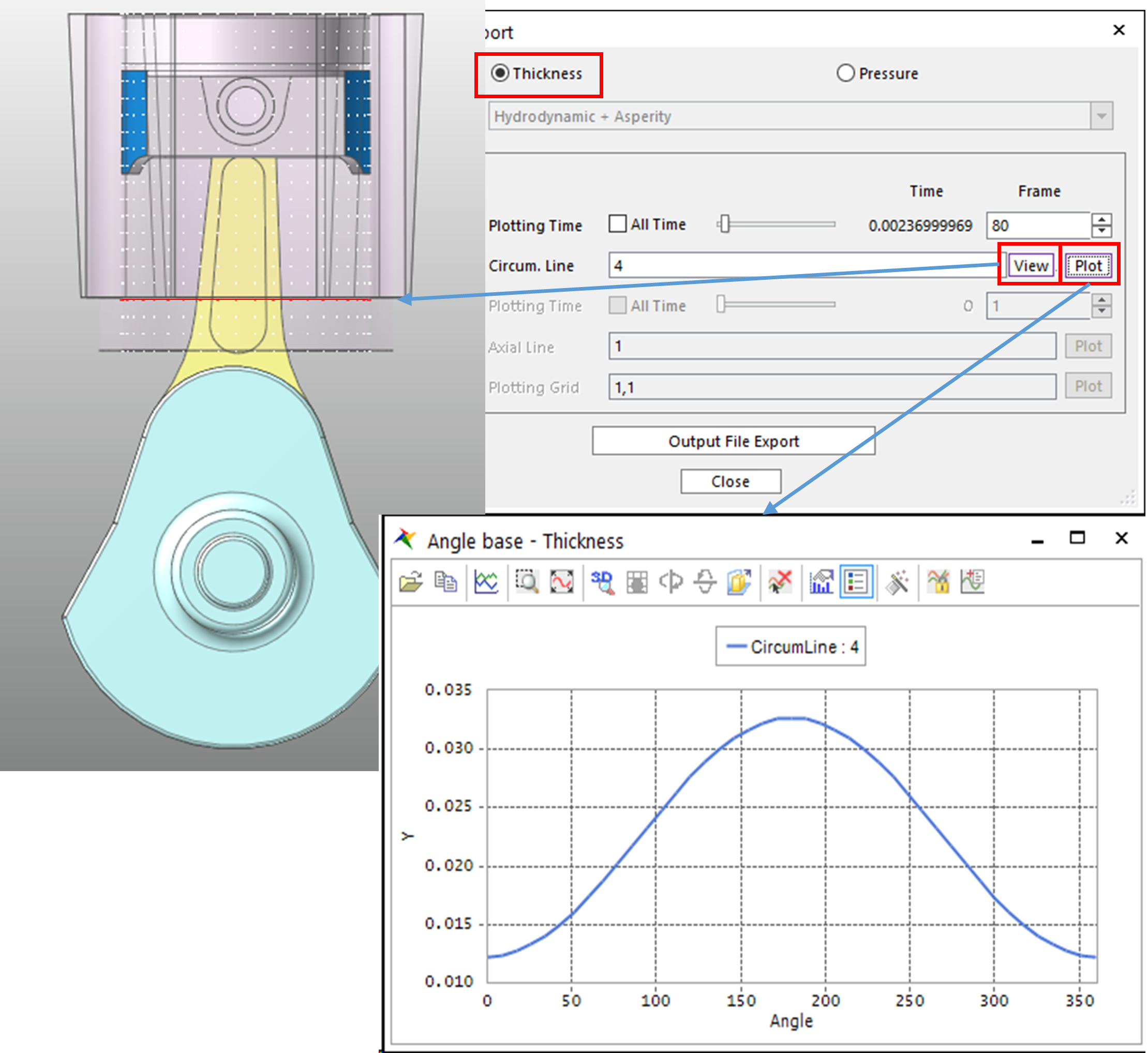
You can see that the thickness of the oil film changes along the 4th line.
Select Pressure and click Plot under the same state as before.
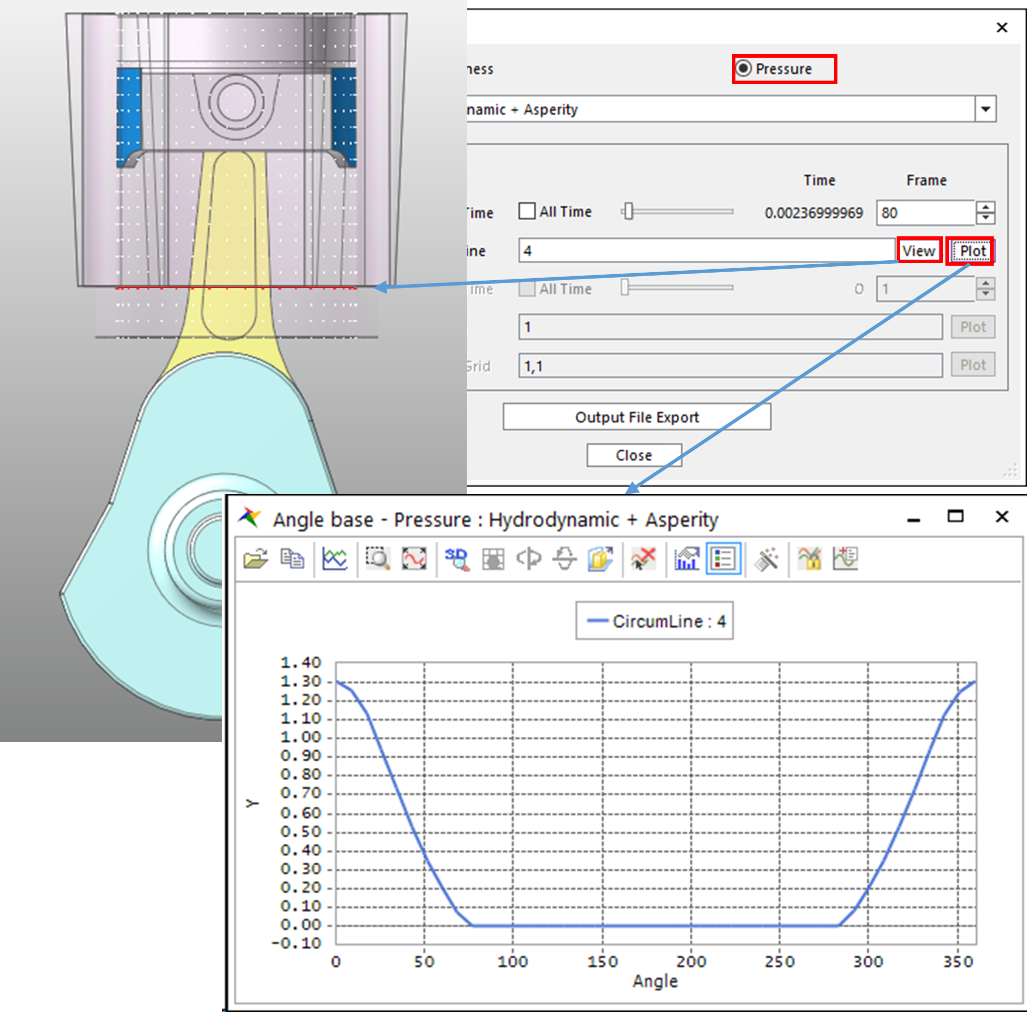
You can see that the pressure increases at the point where the oil film is thin.
9.5.4. Analyzing Piston Lubrication with RFlex Bodies
9.5.4.1. Task Objectives
In this chapter, the cylinder and the piston in the previously defined rigid model are defined as RFlex bodies and the piston lubrication is analyzed considering the deformation.
9.5.4.2. Estimated Time to Complete This Task
30 minutes
9.5.4.3. Creating RFlex Bodies
Click the G-Manager function in the G-Manger group under the Flexible tab.
From the Working Window, select Cylinder Body to display the G-Manager dialog window.
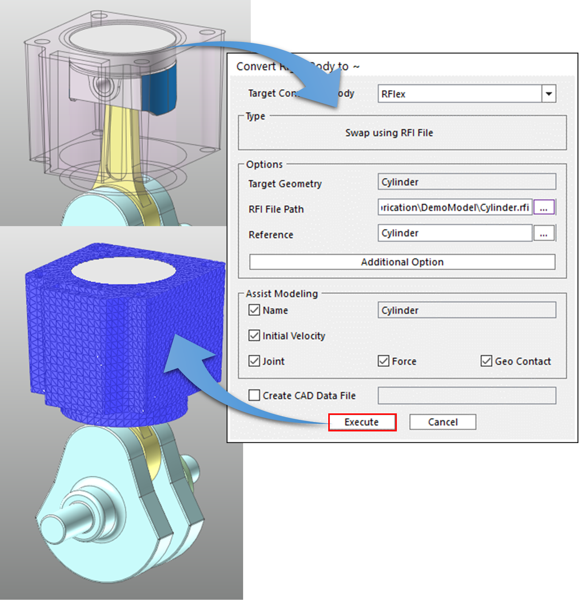
Select RFlex for the Target Converting Body field and set the Type field to Swap using RFI File.
For the purpose of this tutorial, the RFI file is provided in the <InstallDir>\Help\Tutorial\Toolkit\EHD folder.
Set the RFI File Path field to Cylinder.rfi.
Use Cylinder for the Reference field.
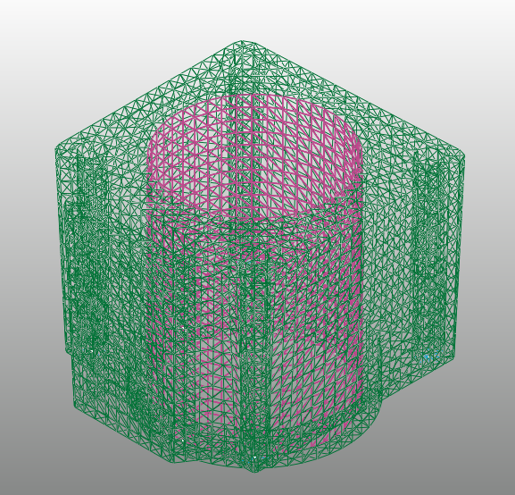
Click the Execute button in the G-Manager dialog window. The Cylinder will be replaced with that of an RFlex Body as shown in the following figure.
Also, for the Piston, use the Piston.rfi file and replace the piston with that of an RFlex Body in the same way as above.
9.5.4.4. Creating PatchSet
From the Working Window, select the Cylinder Body and double-click it.
When you entered the Flex Edit Mode, click the Patch Set function in the Set group under the RFlex Edit tab to create a PatchSet.
From the Patch Set dialog window, click the Add/Remove (Continuous) button and select one of patches placed at the inner side of the cylinder body.
Click Finish Operation from the context menu that appears when you right-click, press the OK button to close the Patch Set dialog window. You will see that SetPatch1 is created.
Click the Exit function to return to the Assembly Mode, select the Piston Body again and double-click it.
To create a PatchSet, click the Patch Set function in the Set group under the RFlex Edit tab.
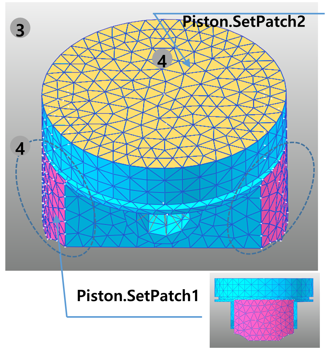
For the Piston Body, create two patch sets, one at the top where the gas explosion pressure will be applied and the other for piston lubrication.
Click the Exit function to return to the Assembly Mode.
9.5.4.5. Defining Modal Pressure Load to Piston
Delete Translational1 used for the rigid body model.
Click the Modal Pressure Load function in the RFlex group under the Flexible tab.
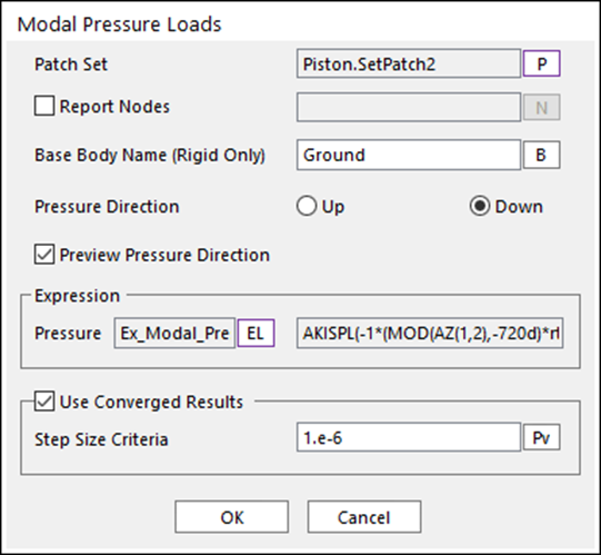
For the patch set, select Piston.SetPatch2 (PatchSet at the top of the piston), which was previously created, from the Modal Pressure Loads dialog window.
Change the Pressure Direction option to Down so that the pressure is applied to the piston.
Click the EL button. From the Expression List dialog window, select the EX_Modal_Pressure field and set the pressure value.
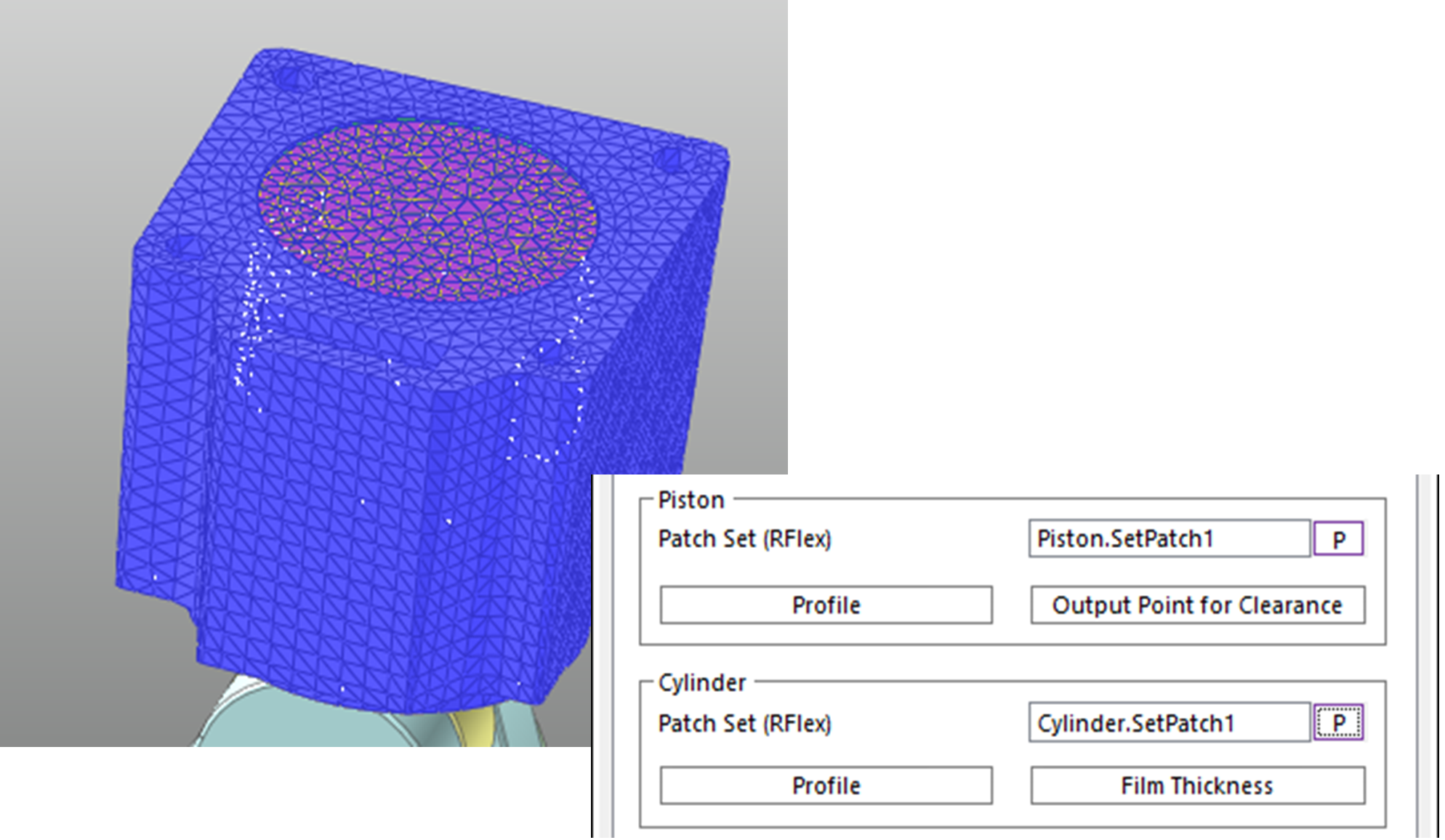
9.5.4.6. Configuring RFlex Body PatchSets for Piston Lubrication
Open the Properties dialog window for Lubrication1.
Enter Patch Sets for the cylinder and the piston respectively.
9.5.4.7. Performing Dynamic Analysis on Piston Lubrication and Checking Its Result
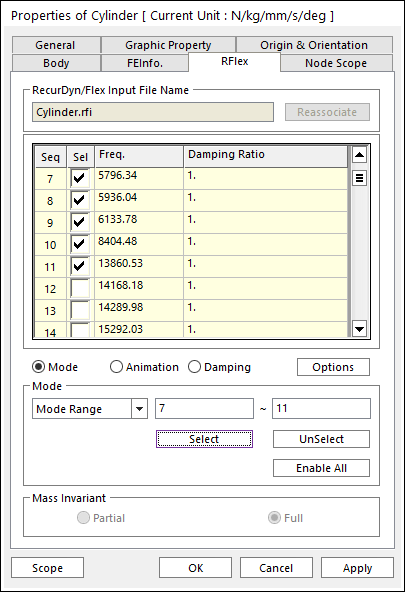
9.5.4.7.1. To reduce the number of RFlex body modes:
10 or more modes exist for each RFlex body. To shorten the analysis time, use only 5 modes for each body.
Right-click Cylinder Body and select Properties in the context menu.
Select the Mode option under the RFlex page in the Properties dialog window for Cylinder Body.
Select Mode Type for the Mode Range and click the UnSelect button to deselect all the modes.
Enter 7 - 11, click the Select button and make sure that 5 consecutive modes are checked starting from the mode no. 7.
Also, for the Piston Body, select only 5 modes in the same way as below.
9.5.4.7.2. To run the simulation for piston lubrication:
Save the model as PistonLubricationEHD_RFlex.rdyn.
On the Analysis tab, in the Simulation Type group, click the Dynamic / Kinematic Analysis function.
The Dynamic/Kinematic Analysis dialog window appears.
Change the End Time field to 0.03 and the Step field to 1000 and click Simulate.
It will take approximately 34 minutes for the analysis.
9.5.5. Analyzing the Results
9.5.5.1. Task Objectives
In this chapter, we will check the results of an analysis performed on the previously defined model.
9.5.5.2. Estimated Time to Complete This Task
10 minutes
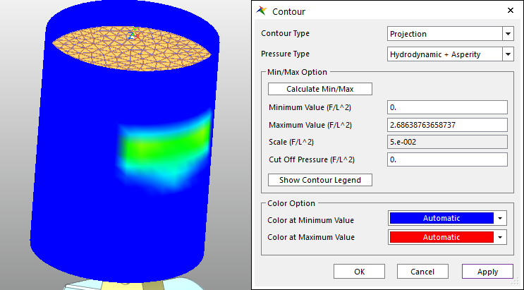
9.5.5.3. Viewing Contour Result
Uncheck the Show All option in the Layer Settings dialog window to hide the cylinder and display only Layer 1.
Right-click Lubrication1 and select Properties in the context menu.
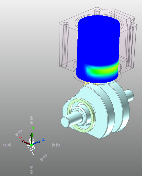
Check the Show Pressure Contour option and click Contour Setting.
Select Hydrodynamic + Asperity for the Pressure Type field to check all the forces of the lubrication and click Apply to check the Contour.
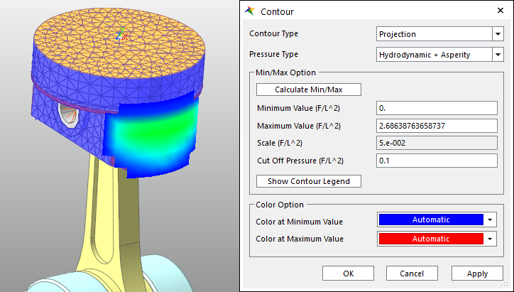
To view only the skirt section of the piston, enter 0.1 in the Cut Off Pressure field in the Contour dialog window and click Apply to check the Contour.
9.5.5.4. Viewing Plot Result
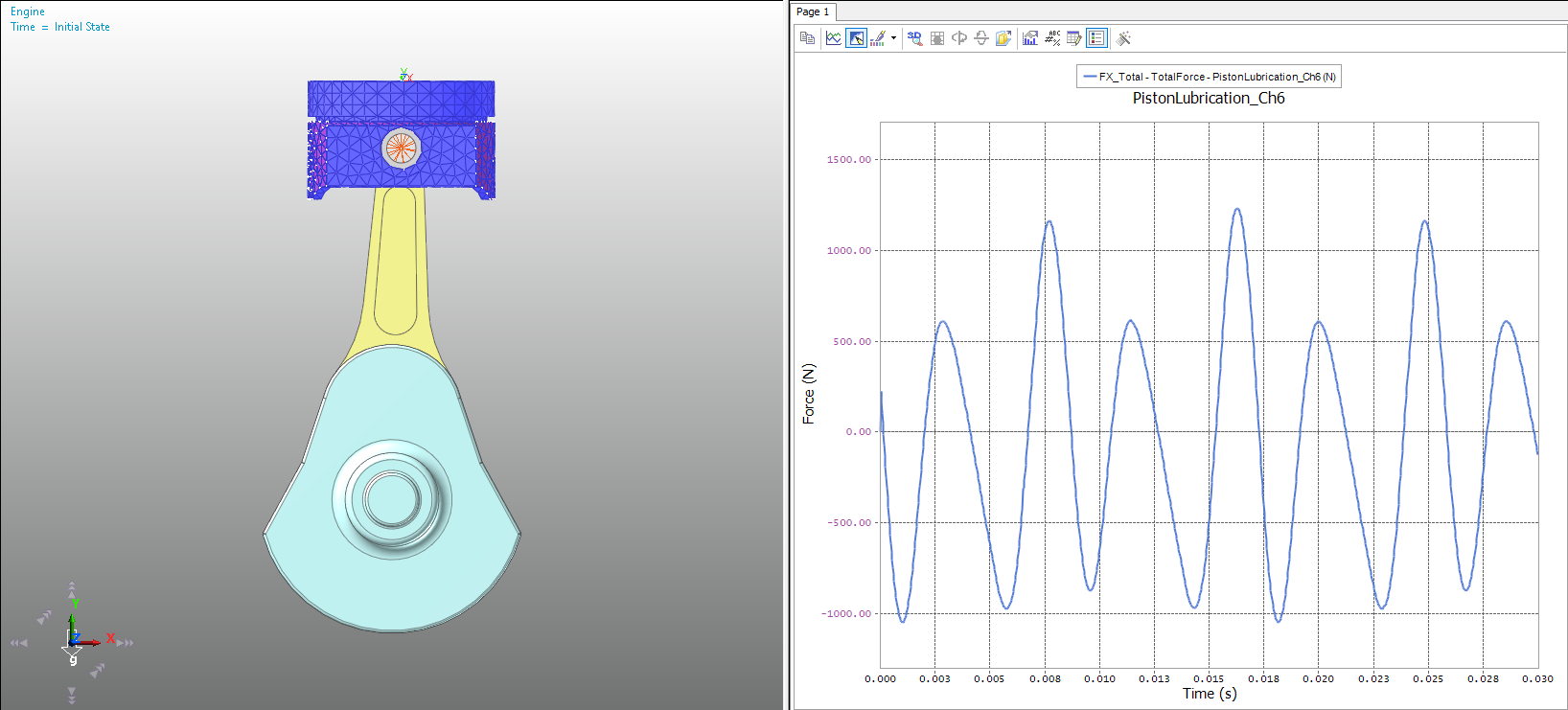
Click the Plot Result function in the Plot group from the Analysis tab.
From the Plot Window, click the Show Upper Windows function in the Windows group from the Home tab.
In the window at the left, click the Load Animation function in the Animation group from the Tool tab. In the widow at the right, select the Force -> PistonLubrication EHD Force -> Lubrication1 -> Total -> FX_Total option in Plot Database Window to draw a plot.
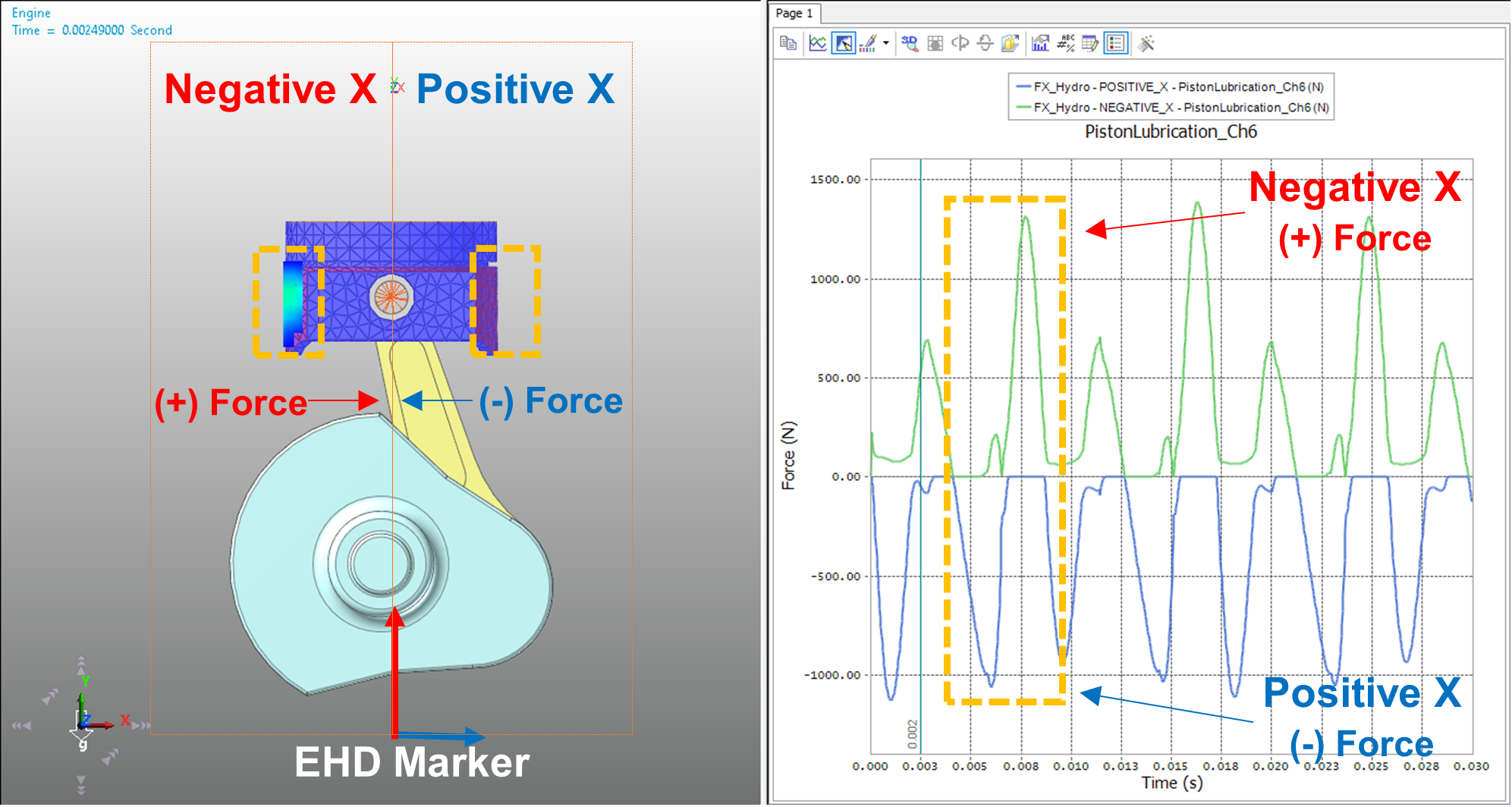
Clear the plot drawn just before. From Plot Database window, select the following two data items to draw them:
Force -> PistonLubrication EHD Force -> Lubrication1 -> HydroDynamicForce -> POSITIVE_X -> FX_Hydro
Force -> PistonLubrication EHD Force -> Lubrication1 -> HydroDynamicForce -> NEGATIVE_X -> FX_Hydro
Click the Add Page function in the Windows group under the Home tab to add a page to the Plot Window. From Plot Database Window, select the following two data items to draw them:
Force -> PistonLubrication EHD Force -> Lubrication1 -> AsperityContactForce -> POSITIVE_X -> FX_Asperity
Force -> PistonLubrication EHD Force -> Lubrication1 -> AsperityContactForce -> NEGATIVE_X -> FX_Asperity
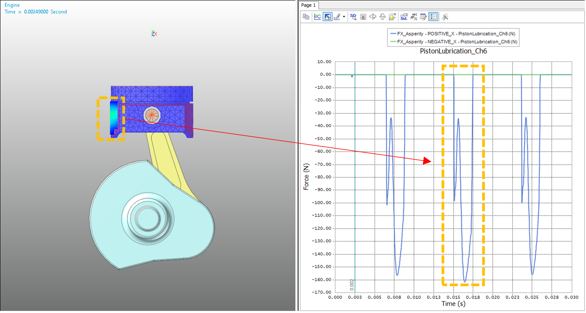
From the plot and contour results, you can check the contact point and the magnitude of the force over time.
9.5.5.5. Checking Oil Film Thickness at Desired Points
Go back to the Modeling Window, right-click Lubrication1 and select Properties from the context menu.
Click Output Point for Clearance in the Properties dialog window for Lubrication1.
To check lubrication depths at the points shown in the figure to the below, set the Output Gap Point dialog window as follows:
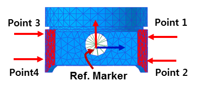
Enter Piston.Marker1 in the Reference Marker field.
Click Add several times to enter information as follows:
1) Height: 14, Angle: 02) Height: -14, Angle: 03) Height: 14, Angle: 1804) Height: -14, Angle: 180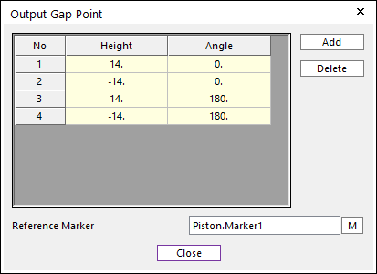
Click Close to close the dialog window.
To check the values, perform the analysis again.
Click the Plot Result function in the Plot group from the Analysis tab.
From the Plot Window, click the Show Upper Windows function in the Windows group from the Home tab.
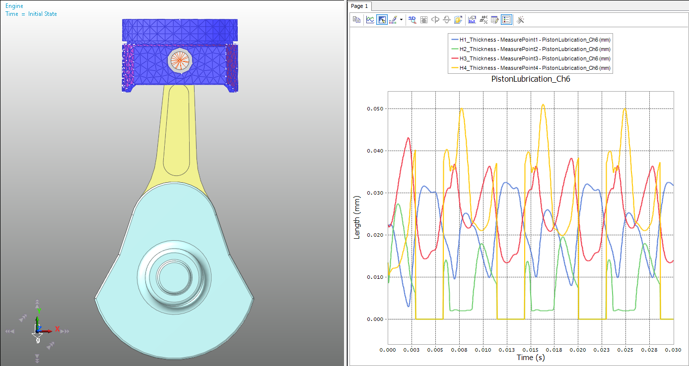
In the window at the left, click the Load Animation function in the Animation group from the Tool tab. In the window at the right, select the 4 data items under the Force -> PistonLubrication EHD Force -> Lubrication1 -> MeasurePoints option in Plot Database Window to draw all of them.
9.5.6. Modifying Piston Profile and Analyzing Piston Lubrication
9.5.6.1. Task Objectives
In this chapter, you will learn how to analyze piston lubrication by changing the piston profile without modifying the previously defined RFlex model.
9.5.6.2. Estimated Time to Complete This Task
10 minutes
9.5.6.3. Modifying Piston Profile
Right-click Lubrication1 and select Properties in the context menu.
Click Profile in the Piston group under the Properties dialog window for Lubrication1.
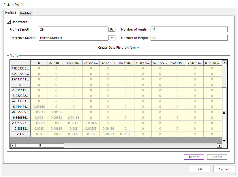
When the Piston Profile dialog window appears, check the Use Profile option and enter values for the parameters to set the profile as follows:
Profile Length: 29
Number of Angle: 44
Reference Marker: Piston.Marker1
Number of Height: 19
From the Piston Profile dialog window, click Create Data Field Uniformly and the data will be generated automatically for each angle and height.
Click Export to export the generated data.
You cannot modify the data in the Piston Profile dialog window. Export the data to a file and use Excel or a text editor to modify the data in the file.
- Click Import to import the ProfileData.csv file provided in this tutorial.(The file path: <InstallDir>\Help\Tutorial\Toolkit\EHD\PistonLubrication)
Click OK in the Piston Profile dialog window to close it as well as to apply the data to the model. Click OK in the Properties dialog window for Lubrication1.
9.5.6.4. Analysis and Comparison
Save the model as PistonLubricationEHD_RFlex2.rdyn.
On the Analysis tab, in the Simulation Type group, click the Dynamic / Kinematic Analysis function.
The Dynamic/Kinematic Analysis dialog window appears.
After verifying the simulation conditions, click Simulate.
Click the Plot Result function in the Plot group from the Analysis tab.
From the Plow Window, import the rplt file, which is the result of previous analysis.
Right-click the Force -> PistonLubrication EHD Force -> Lubrication1 -> AsperityContactForce -> NEGATIVE_X -> FX_Asperity data from Plot Database Window and click Multi Draw from the context menu.
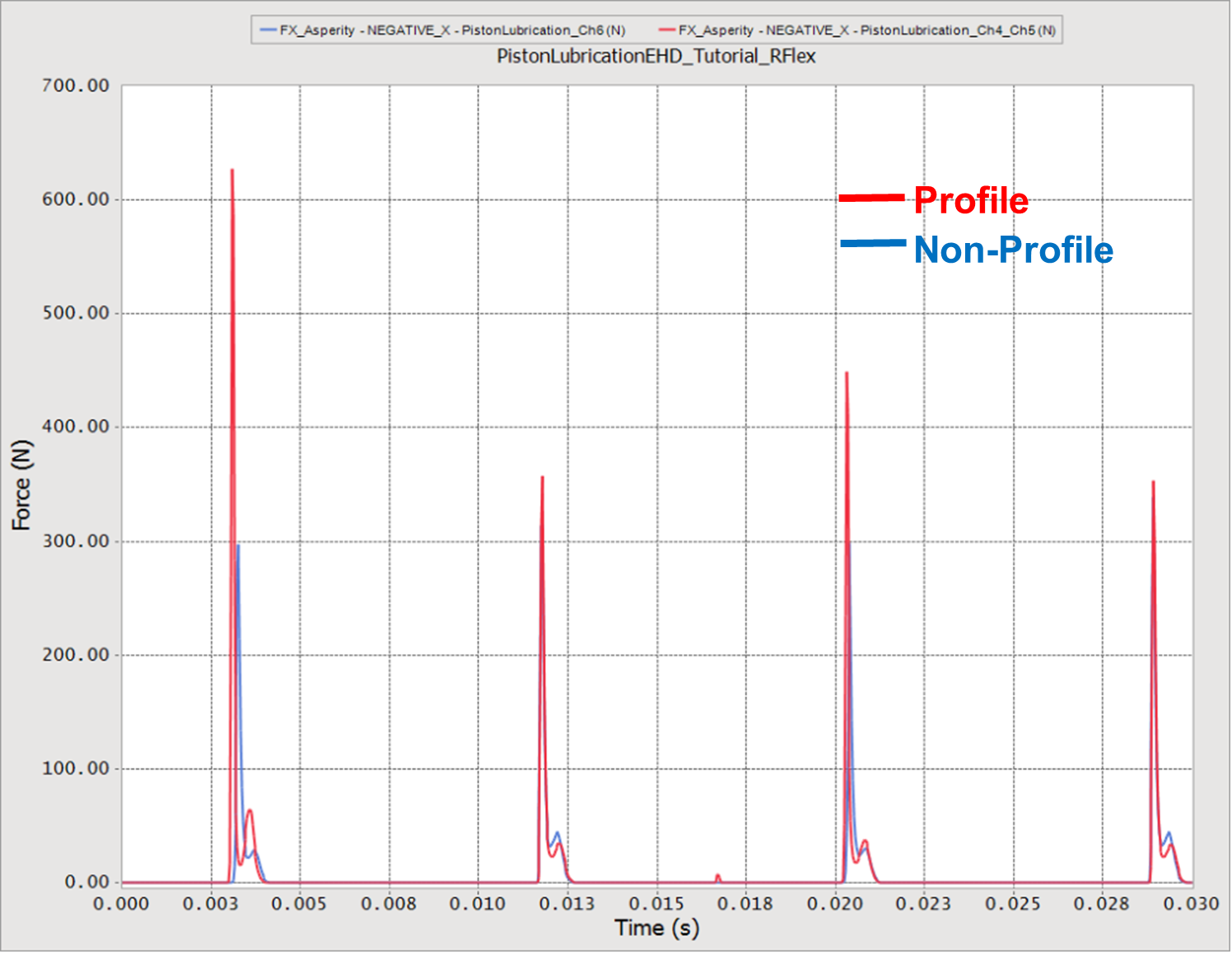
You will see that the result changes according to the piston profile.