1.1. 3D Slider Crank Tutorial (Professional)

1.1.1. Getting Started

1.1.1.1. Objective

In this introductory tutorial, you will learn how to:

• Set up a model with the correct units and environment

• Create bodies with geometric detail

• Add joints and associated input motions

• Analyze the model to investigate the effects of motion and forces on it.

• Communicate the results of your simulation as:

  • X-Y plots

  • Animations that can be played interactively within RecurDyn

  • AVI files that can be inserted into PowerPoint presentations

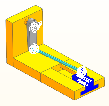
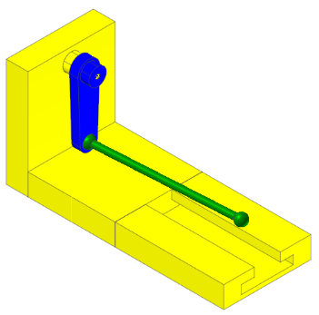
The target model is a 3D slider-crank mechanism. This mechanism is used to convert an input rotary motion to an output translational motion. You will see how the combination of moving bodies and four kinematic joints can produce a complex relationship between the input and output motions.

1.1.1.2. Audience

This tutorial is an excellent starting point for the engineer who is using RecurDyn for the first time. The basic tasks that are needed for all simulations are explained carefully.

1.1.1.3. Prerequisites

Because this is an introductory tutorial, we assume that you have no prior experience with RecurDyn. We assume that you have a basic knowledge of physics.

1.1.1.4. Procedures

The tutorial is comprised of the following procedures. The estimated time to complete each procedure is shown in the table.

Procedures	Time (minutes)
Simulation environment setup	5
Geometry creation	35
Joint creation	10
Analysis	5
Animation/AVI	10
Plotting	10
Total	75

1.1.1.5. Estimated Time to Complete

75 minutes

1.1.2. Setting Up Your Simulation Environment

1.1.2.1. Task Objective

Learn how to set up the simulation environment, including units, materials, gravity, and the working plane.

1.1.2.2. Estimated Time to Complete

5 minutes

1.1.2.3. Starting RecurDyn

1.1.2.3.1. To start RecurDyn and create a new model:

1. On your Desktop, double-click the RecurDyn icon. RecurDyn starts up and the Start RecurDyn dialog box appears.

   

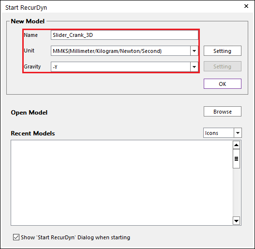
2. Enter the name of the new model as Slider_Crank_3D.

3. Change Unit to MMKS. (Millimeter/Kilogram/Newton/Second)

4. Gravity is the Default (-Y) setting.

5. Click OK.

Tip

Other ways to create a new model

If you want to create a new model in RecurDyn, you can do one of the following:

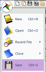
• In the Quick Access Toolbar, click the New.

• From the File menu, click New.

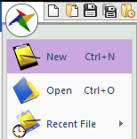
• Use the shortcut key (Ctrl+N).

Tip

Allowed Characters for Model Name

You cannot use spaces or special characters in the model name. You can use the underscore character _ to add space to improve the readability of the name.

Tip

Create User Unit Setting

You can create user-defined units when you need custom unit settings.

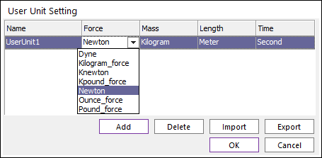
• Click Setting next to Unit.

• User Unit Setting dialog will appear. You can define units regarding Force, Mass, Length, and Time.

  

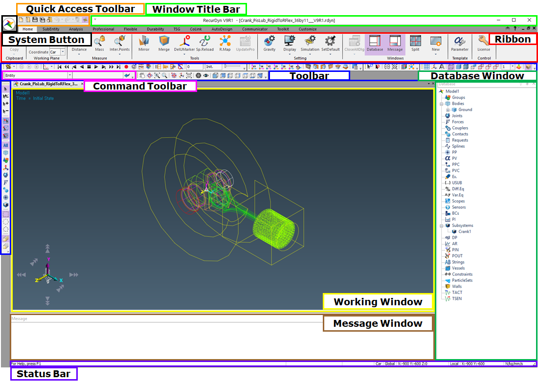
1.1.2.4. Understanding the Interface

The RecurDyn interface consists of several basic areas as shown in the below figure. You can turn on and off the display of any areas and rearrange the areas any way you want. Each area is explained below.

1.1.2.4.1. Using the Ribbon menu

The Ribbon menu provides you with all the tools you need to create a model, including the geometries, constraints, and motions. It divides the tools into subcategories to make it easier for you to find the tools.

1.1.2.4.2. To select a tool:

1. Click the tab, such as SubEntity or Professional. The set of tools in that category appears.

2. Click the desired tool.

1.1.2.4.3. Using the Database Window

You can view all the data and entities in your model using the Database Window. In addition, you can:

• View and change the properties of each entity.

• Make constraints and forces inactive and reactivate.

• Change the display modes of individual bodies.

• Change to the edit mode of subsystems, bodies, and profiles.

• Check information of lower-level entities by clicking + button in front of entities.

1.1.2.4.4. To view the entities in your model:

Click the + in front of an entity in the database window.

1.1.2.4.5. Using the Working Window

The Working window is where you build your model. You can use the tools to zoom and rotate your model and set the working plane on which you build your model.

1.1.2.4.6. Using the Working Plane

Working plane is where you modify entities. You can modify the working plane setting using the working plane toolbar. Grid changes according to axis of working plane. Status of working plane can affect forms and directions of entities you work on

1.1.2.4.7. Using Command Toolbar

Command Toolbar is located at the top of the window. It is composed of those two modeling toolbars below and helps you create your model:

• The Creation Method Toolbar sets the options for the current operation.

• The Input Window Toolbar lets you enter coordinates or a parametric point name and value, depending on the required input.

  

1.1.2.4.8. To use the toolbars together to create your model:

1. Select an entity to create, such as a cylinder.

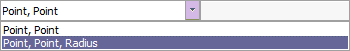
2. From the Creation Method Toolbar, select a creation method, such as Point, Point, Radius.

3. Enter the first point in the Input Window Toolbar.

4. Press Enter or click. (right side of the command toolbar).

5. Enter the second point in the Input Window Toolbar.

6. Press Enter or click.

1.1.2.4.9. Status Bar

The Status bar provides information about the state of your model.

1.1.2.4.10. System Modes in RecurDyn

There are four modes in which you can work in RecurDyn:

• Model Edit Mode

  • Work on the entire model. Let you create objects in your model at the top level in the model hierarchy.

  • You can work on every entity.

• Subsystem Edit Mode

  • Work on the all of the entities in a subsystem.

  • Let you create objects in your model that belong to a logical subsystem in your model. A subsystem can contain a group of entities that are created by using the process automation of a RecurDyn toolkit, such as a belt, chain, or track assembly.

• Body Edit Mode

  • Edit geometry of bodies.

  • Edit a particular entity in your model, such as ground, a link, or force.

By default, RecurDyn is in model-editing mode. You switch between the modes depending on the operations that you want to perform. In this tutorial, you’ll switch to body-editing mode to edit the ground and then you will switch to the profile-editing mode as needed to create geometry.

1.1.2.4.11. Changing System Modes:

• In the Database window, right-click an entity, and from the menu that appears, click Edit.

• In the Working window, double-click a subsystem, body, or profile geometry.

• Click on one of the mode tools on the toolbar.

1.1.2.5. Changing the Gravitational Force Direction

In this tutorial, you will change the gravitational force of the -Z directions.

1.1.2.5.1. To change the gravitational force direction:

1. From the Setting group in the Home tab, click the Gravity function.

   

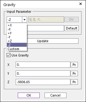
2. Choice direction of the -Z and click Update.

3. Click OK.

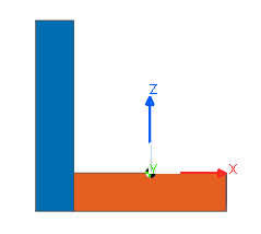
1.1.2.6. Changing the Working Plane

You will now use the Working Plane tool on the toolbar to change the current working plane into the XZ plane about the inertia reference frame.

1.1.2.6.1. To toggle Grid on working plane

If you turn on Grid, you can check the status of working plane

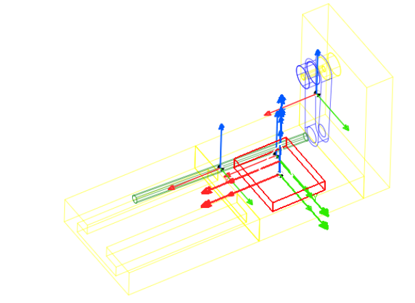
• Toggle the Grid On/Off tool in Render Toolbar. Grid will appear in Working Window.

  

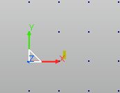
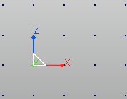
1.1.2.6.2. To change the working plane:

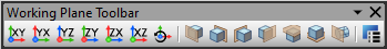
1. In View Control Toolbar, click the combo box next to the Working Plane Change (Axis) tool.

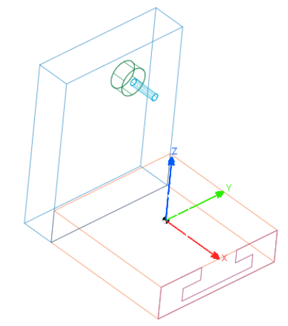
2. Select the Change to XZ tool. Working Plane and Inertia Reference Frame will be rotated to XZ Plane as shown below.

   

   The Working Plane Change (Axis) function can only change the working plane about the Inertia Reference Frame. If you want to change the working plane about another plane, see the Tip below.

   

Tip

How to select the working plane

• From View Control Toolbar, click the Working Plane Setup tool. The Working Plane Setup dialog box appears. In this dialog, you can set the options about Plane and Grid.

  

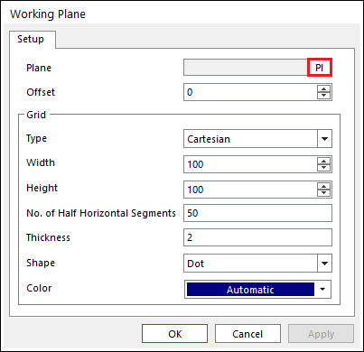
• By clicking PI, you can set the user-defined Working Plane. You can define it by using two method below.

• Using user-defined Marker Plane: You can set the Working Plane to XY, YZ, XZ Plane of user-defined General Marker.

• Using Face of user Geometry: You can set the Working Plane to Face of CAD Geometry in model.

• In the dialog, you can modify the status of grid (Type, Size, Color etc) shown in Working Window.

Tip

Rotating user-defined Working Plane

• You can change the direction of user-defined working plane using Working Plane Change function.

  

1.1.3. Creating Geometry

1.1.3.1. Task Objective

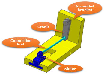
In this chapter, you will create geometry to define the 3D slider crank, which consists of:

• Grounded bracket

• Crank

• Connecting rod

• Slider bodies

  

1.1.3.2. Estimated Time to Complete

35 minutes

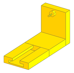
1.1.3.3. Modeling the Grounded Bracket

In this section, you create geometry to define the grounded bracket. You will create the bracket using two boxes, two cylinders, and two extrusions. This will also introduce you to the basics of using the toolkits to create geometry.

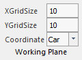
1.1.3.3.1. To change the Grid Size

• From the Home tab in the Working Plane, input 10 and press Enter key. (Also, you can modify it in Working Plane dialog mentioned in chapter 2.)

  

1.1.3.3.2. To change Body Edit Mode to create a bracket

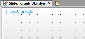
• From Professional tab in the Marker and Body group, click the General function for entering body edit mode. Body1@Slider_Crank_3D is marked on the top left of working window as shown at bottom.

  

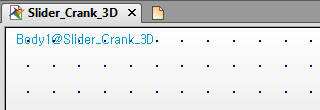
  It means that you entered the edit mode of Body1 Entity in Slider_Crank_3D Model. All created geometries in this edit mode are considered as one rigid body Body1.

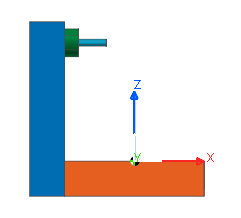
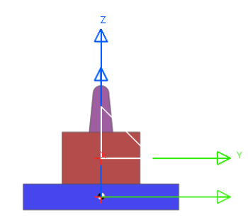
1.1.3.3.3. To create Box Geometry

1. From Geometry tab in the Marker and Geometry group, click the Box function.

2. Set Creation Method to Point, Point, Depth.

3. Create Boxes using following information. You can click on the Working Window or use Input Window Toolbar. (For detailed information, refer to Chapter 2.)

   • Point1: 100, 0, -50

   • Point2: -100, 0, 0

   • Depth: 200

4. Repeat Steps 1-3 using following information.

   • Point1: -150, 0, 200

   • Point2: -100, 0, -50

   • Depth: 200

   Box geometries are created as shown at bottom.

   

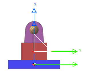
1.1.3.3.4. To create the cylinder geometry:

Since you will create two cylinders at one time you will use the Auto Operation mode to automatically remain in the cylinder creation mode. The Auto Operation mode can be used with any input command and it can save a substantial amount of time when you are creating many entities of the same type.

1. Click on the Auto Operation tool to activate the Auto Operation input mode.

2. From the Solid and Marker group in the Ground tab, click the Cylinder function.

3. Set the Creation Method to Point, Point, Radius.

4. In the Working window, click these points and input a depth for both cylinders in the Input Window toolbar:

   Cylinder 1:

   • Point1: -100, 0, 170

   • Point2: -80, 0, 170

   • Radius: 20

   Cylinder 2:

   • Point1: -80, 0, 170

   • Point2: -40, 0, 170

   • Radius: 5

5. Click on the Auto Operation tool again to exit the Auto Operation input mode. (Click on the Esc key to exit the Cylinder input tool.) The cylinders you created should look like the following:

   

Tip

How to modify the geometry properties

If you want to modify the parameters of geometry, you can modify them by using the Properties dialog box.

• You can open Properties dialog by using one of three method below.

  • In Database Window, right-click the entity and click Properties.

  • Select the entity in Working Window, click Properties in right-click menu.

  • In Database Window or Working Window, select entity and click P key on the keyboard which is the shortcut for Properties

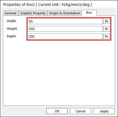
The following shows the properties for a box and a cylinder.

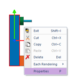
• Properties dialog is shown which can modify parameters.

  • For example, you can edit Width, Height, Depth in Box page in Properties of Box2.

  • Clicking OK/Apply will apply the modified value.

  

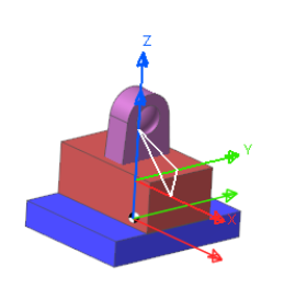
1.1.3.3.5. To create outline for extrusion

1. In View Control Toolbar, click the Change to YZ tool.

   

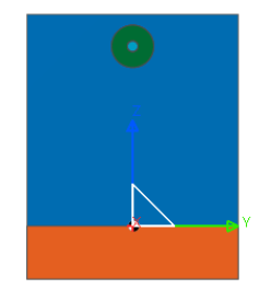
2. Click the Outline function from Curve group in the Geometry tab.

3. Input Point values using information below.

   Point	X	Y,	Z
   1	100	-100,	0
   2	100	-100,	-50
   3	100	100,	-50
   4	100	100,	0
   5	100	30,	0
   6	100	30,	-20
   7	100	60,	-20
   8	100	60,	-40
   9	100	-60,	-40
   10	100	-60,	-20
   11	100	-30,	-20
   12	100	-30,	0
   13	100	-100,	0

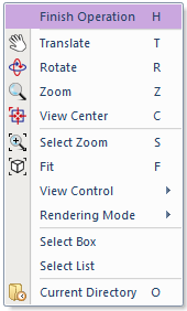
4. When you finished inputting all 13 point values, right-click on the working window and click Finish Operation in the pop-up menu.

   

   Outline1 is created as shown below. (If geometry of Outline1 is not as same as the picture below, open the properties dialog and modify the point values.)

   

1.1.3.3.6. To create Curve Sweep

1. Click the Fill Surface function from Curve tab in the Geometry group.

2. Select Outline1. FilledSurface1 is created.

3. Click the Extrude Solid function from Geometry tab in the Solid group

4. Set the Creation Method to Surface, Direction, Distance.

5. Create extrude using following information.

   • Surface: FilledSurface1

   • Direction: 1,0,0

   • Distance: 250

   Extrude1 is created.

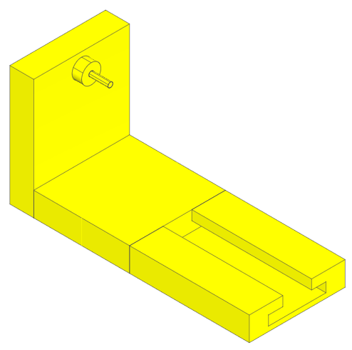
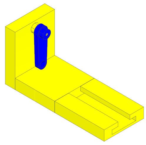
Finished Bracket will look like a picture shown at bottom. Check if there is a problem by changing a model view.

Tip

Changing Model View

You can use View Control Toolbar to change the view.

• Translate or Rotate the model view by using methods below.

  • Click the Translate tool in View Control Toolbar to translate the model view. (Shortcut for this operation is T key)

  • Click the Rotate tool in View Control Toolbar to rotate the model view. (Shortcut for this operation is R key).

• Zoom the model view using methods below.

  • Click the Select Zoom tool in View Control Toolbar, drag the area you want to zoom. (Shortcut for this operation is S key).

  • Zoom the model view by turning Mouse Wheel button.

1.1.3.3.7. To exit body edit mode.

In Body Edit Mode, you have created all of geometries for Bracket. Now we change to Model edit mode by exiting Body Edit Mode.

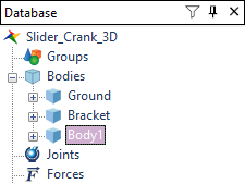
• Click the Exit function from Exit group in the Geometry tab. Upper-Left side of Working Window, you can see the title Slider_Crank_3D.

  

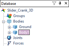
• In Database Window, you can check that Body1 is created which contains Bracket Geometry.

  

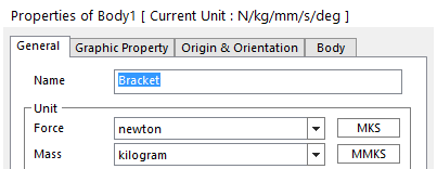
1.1.3.3.8. To change name and color of the Body.

1. Open Properties dialog of Body1.

2. Click General page in Properties dialog.

3. Change Name to Bracket.

   

4. Click Graphic Property page.

   

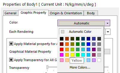
5. Change Color to Yellow.

6. Click OK.

   

1.1.3.4. Modeling the Crank Body

You will create Link, Ellipsoid and Cylinder geometry and do Boolean operation to create Crank Body.

1.1.3.4.1. To change the working plane

• Select the Change to YZ tool in View Control Toolbar.

1.1.3.4.2. To create the crank body:

1. From the Body group in the Professional tab, click the Link function.

2. Set Creation Method to Point, Point, Depth.

3. Click these points:

   • Point1: 0, 0, 30

   • Point2: 0, 0, 170

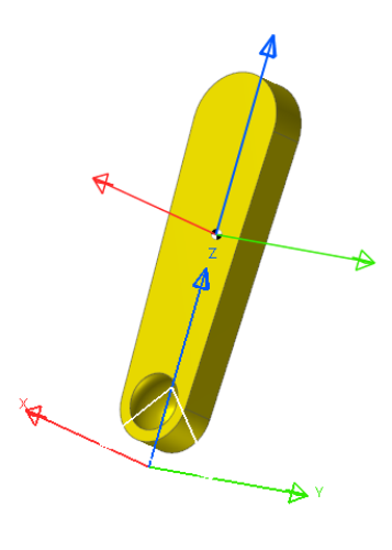
   • Depth: 20

   Your link geometry should now look like the one shown below.

   

1.1.3.4.3. To change the name of the body:

1. Right-click the working window over the model Body1, then click Properties.

2. Click the General page in Properties dialog.

3. Change the body name from Body1 to Crank.

4. Click OK.

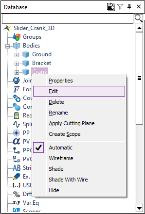
1.1.3.4.4. Modifying the Link Geometry

You will modify Property of Link geometry after entering Body Edit Mode of Crank.

1. In the Database Window, right-click Crank and click Edit. After entering edit mode of Crank body, the Link geometry is now the only geometry in the Working Window.

   

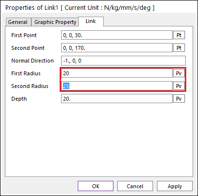
2. Open the Properties dialog of Link1, change the values as below.

   • First Radius: 20

   • Second Radius: 25

     

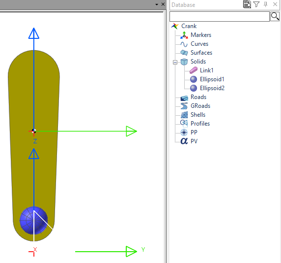
1.1.3.4.5. To create Ellipsoid geometry

1. Click the Ellipsoid function from Marker and Geometry group in the Geometry tab.

2. Input values using information below.

   • Point: 0,0,30

   • Distance: 15

3. Repeat 1-2 steps using information below.

   • Point: 5,0,30

   • Distance: 15

     

1.1.3.4.6. To do Boolean Unite

You will create Ellipsoid geometry and unite it with Link geometry by using Boolean Unite.

1. Click the Unite function from the Boolean group in the Geometry tab.

2. Select the Link1 geometry and then the Ellipsoid1 geometry. Selected two geometries (Link1 and Ellipsoid1) disappear and Unite1 is created.

1.1.3.4.7. To do Boolean Subtract

You will scoop out the part of Link geometry with Ellipsoid geometry using Boolean Subtract.

1. Click the Subtract function from Boolean group in the Geometry tab.

2. Select Unite1 and then select Ellipsoid2. Selected two geometries (Unite1 and Ellipsoid2) disappear and Subtract1 is created.

   

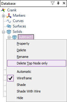
Tip

How to undo a Boolean Unite Operation

Entity created by Boolean operation has hierarchy in Database Window. Inside of hierarchy, there is history of Boolean operation.

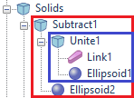
You can restore the united geometry to its previous state using the Delete Top Node only menu shown below. In this case, the top node would be the Unite1.

1.1.3.4.8. To create a cylinder:

1. Select the Change to XZ tool in View Control Toolbar.

2. Click the Cylinder function from Marker and Geometry group in the Geometry tab.

3. Set the Creation Method to Point, Point, Radius.

4. Input values using information below.

   • Point1: 10, 0, 170

   • Point2: 30, 0, 170

   • Radius: 20

     

1.1.3.4.9. To exit the edit mode of crank body

• Click the Exit function from the Exit group in the Geometry tab.

1.1.3.4.10. To change the color of crank body

• Open the Properties dialog of Crank body and change Color to Blue.

  

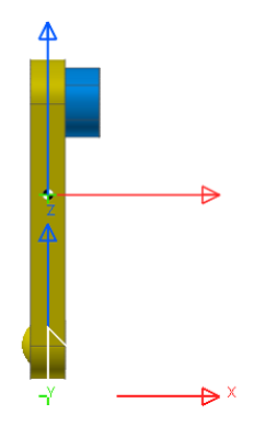
1.1.3.4.11. To translate the crank body

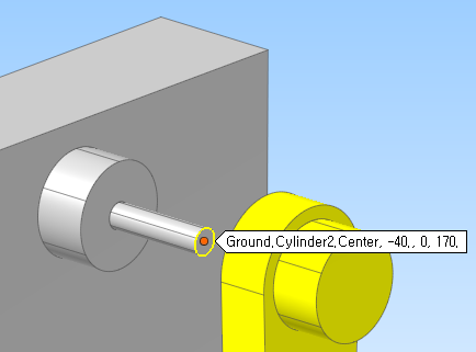
Crank is separated from Bracket. You will measure the distance between Crank and Bracket and translate Crank body according to the result.

1. Click the Distance function from Measure group in the Home tab.

2. When Distance dialog appears, click Pt button located next to First Point and select as picture shown below.

3. Click Pt located next to Second Point and select as picture shown below.

4. Click Calculate. Result of Distance Measure is 70.

   

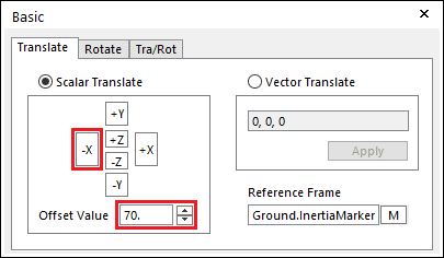
5. Click the Basic Object Control tool in Advanced Toolbar. When the Basic Object Control dialog appears, change Offset Value to 70 in Translate page.

6. Select Crank in the Working Window.

7. After Crank is selected, click -X in the Basic Object Control dialog.

8. Close the Basic Object Control dialog.

   

1.1.3.5. Creating the Connecting Rod

Now you will create the connecting rod by creating a cylinder and two ellipsoids and then unite them with Boolean operations.

1.1.3.5.1. To create the cylinder:

1. From the Body group in the Professional tab, click the Cylinder function.

2. Set the Creation Method to Point, Point, Radius.

3. Create the cylinder body:

   • Point1: -60, 0, 30

   • Point2: 290, 0, 50

   • Radius: 7

1.1.3.5.2. To change name of the body

1. Open the Properties dialog of Body1.

2. Click General page in the Properties dialog.

3. Change Name to Connecting_Rod.

4. Click OK.

1.1.3.5.3. To create Ellipsoid Geometry

1. In Database Window, right-click Connecting_Rod and click Edit. After entering edit mode of Connecting_Rod body, the Cylinder geometry is now the only geometry in the Working Window.

2. From the Marker and Geometry group in the Geometry tab, click the Ellipsoid function.

3. To create the ellipsoid geometry, input values using information below.

   • Point: -60, 0, 30

   • Distance: 13

4. Repeat the steps from 2 to 3 by referring below values.

   • Point: 290, 0, 50

   • Distance: 13

1.1.3.5.4. To do Boolean Unite

After creating Ellipsoid geometry, you will unite Cylinder Geometry by using Boolean Unite. If you don’t unite those geometries, RecurDyn will calculate the unnecessary mass of overlapped area.

1. Click the Unite function from the Boolean group in the Geometry tab.

2. Select Cylinder1 and then select Ellipsoid1. Selected two geometries (Cylinder1 and Ellipsoid1) disappear and Unite1 is created.

3. Click the Unite function again from the Boolean group in the Geometry tab.

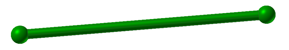
4. Select Unite1 and then select Ellipsoid2. Unite2 is created as shown below.

   

1.1.3.5.5. To exit body editing mode

• Click the Exit function from the Exit group in the Geometry tab.

1.1.3.5.6. To change color of Connecting_Rod

• Open the Properties dialog of Connecting_Rod Body and change Color to Green.

  

1.1.3.6. Modeling the Slider

To model the Slider body, you will create a base box, an upper center box, and link geometry, and then subtract a sphere from the link to make a contacting point with the connecting rod.

1.1.3.6.1. To change working plane

• Select the Change to YZ tool in View Control Toolbar.

1.1.3.6.2. To create the box:

1. From the Body group in the Professional tab, click the Box function.

2. Set the Creation Method to Point, Point, Depth.

3. Create the box geometry:

   • Point1: 0, -60, -20

   • Point2: 0, 60, -40

   • Depth: 100

The box should appear as shown below. You may need to rotate the model to see the box (type R key in the Working window) and you may need to set the rendering mode back to Wireframe with Silhouettes if you changed it earlier to Shade (from the View Control Toolbar, point to Rendering Mode, and click the Wireframe with Silhouettes tool).

1.1.3.6.3. To change the body name

1. Open the Properties dialog window of Body1.

2. Click General page in the Properties dialog.

3. Change Name to Slider.

4. Click OK.

1.1.3.6.4. To add a box to the Slider body:

1. Enter the Body Edit Mode of Slider.

2. In the Marker and Geometry group in the Geometry tab, click the Box function.

3. Set the Creation Method to Point, Point, Depth.

4. Create box geometry:

   • Point1: 0, -30, 20

   • Point2: 0, 30, -20

   • Depth: 100

     

1.1.3.6.5. To add link geometry to the Slider body:

1. From the Marker and Geometry group in the Geometry tab, click the Link function.

2. Set the Creation Method to Point, Point, Depth.

3. Create the link geometry:

   • Point1: 0, 0, 50

   • Point2: 0, 0, -10

   • Depth: 20

   The link should appear as shown next.

4. Modify the link geometry (In the Database Window, right-click Link1, point to Properties, and then click the Link page):

   • First Radius: 20

   • Second Radius: 25

     

1.1.3.6.6. To create ellipsoid geometry:

1. From the Marker and Geometry group in the Geometry tab, click the Ellipsoid function.

2. Create an ellipsoid geometry:

   • Point: 0, 0, 50

   • Distance: 15

3. Repeat 1-2 step using information below.

   • Point: -5, 0, 50

   • Distance: 15

     

1.1.3.6.7. To do Boolean Unite

After creating Ellipsoid geometry, you will unite it with Link geometry by using Boolean Unite.

1. Click the Unite function from the Boolean group in the Geometry tab.

2. Select Link1 and then select Ellipsoid1. Selected two geometries (Link1 and Ellipsoid1) disappear and Unite1 is created.

1.1.3.6.8. To do Boolean Subtract

You will scoop out Ellipsoid geometry from united geometry by using Boolean Subtract.

1. Click the Subtract function from the Boolean group in the Geometry tab.

2. Select Unite1 and then select Ellipsoid2. Selected two geometries (Unite1 and Ellipsoid2) disappear and Subtract1 is created.

   

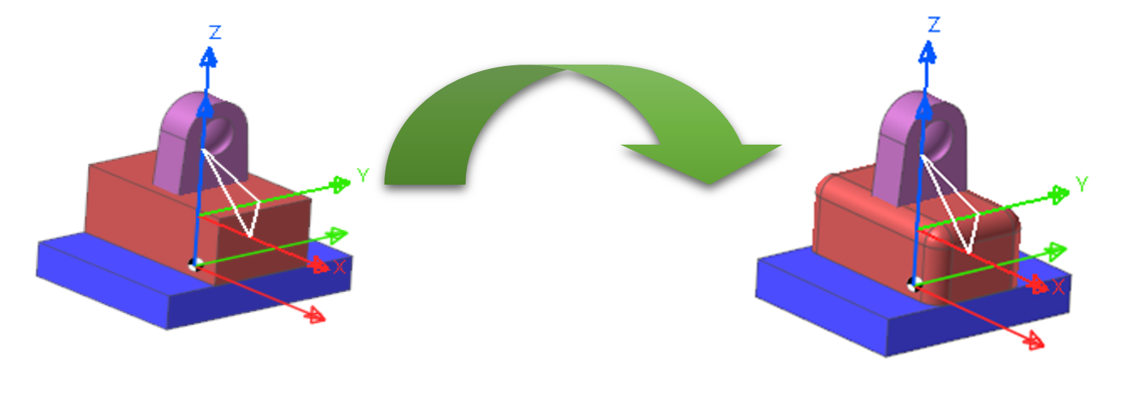
1.1.3.6.9. To fillet the edges of the upper box geometry:

1. From the Local group in the Geometry tab, click the Fillet function.

2. Select the upper Box. The Fillet Operation dialog box appears.

3. Click Add and select the 8 edges of the Box except for the bottom edges of the Box as shown in the picture below. (MultiEdge is the Select Option, so you can select multiple edges at once.)

4. After selecting all 8 edges, right-click on the working window and click Finish Operation in the pop-up menu.

5. The edges from faces you select appear in the Fillet Operation dialog box, as shown below.

   

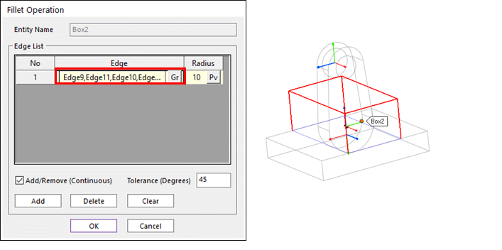
6. Change the radius for each edge to 10, as shown in the Fillet Operation dialog box above.

7. Click OK. The geometry changes as shown below.

   Tip

   Undoing Local operation is same as Boolean Operation.

   

1.1.3.6.10. To do Boolean Unite

• Unite every geometry you worked on with Unite.

1.1.3.6.11. To exit the edit mode of slider body

• Click the Exit function from the Exit group in the Geometry tab.

1.1.3.6.12. To change color of slider body

• Open the Properties dialog of Slider body and change Color to Grey.

  

1.1.3.6.13. To change Working Plane

• Select the Change to XZ tool in View Control Toolbar.

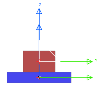
1.1.3.6.14. To translate the slider body

1. Click the Basic Object Control tool in Advanced Toolbar. When the Basic Object Control dialog appears, change Offset Value to 300 in Translate page.

2. Select Slider in the Working Window.

3. After Slider is selected, click +X in the Basic Object Control dialog. Slider is translated by 300mm along +X direction.

4. Close the Basic Object Control dialog.

   

1.1.3.7. Saving Your Model

1. From the File menu, click Save.

   

2. Decide saving location and save file name.

3. Click OK to save.

1.1.4. Creating Joints

1.1.4.1. Task Objective

In this chapter, you will create several joints. You will create a:

• Revolute joint between the Grounded Bracket and the Crank

• Spherical joint between the Crank and the Connecting Rod

• Spherical joint between the Connecting Rod and the Slider

• Translational joint between the Slider and the Grounded Bracket

You will also define the input motion of the crank.

1.1.4.2. Estimated Time to Complete

10 minutes

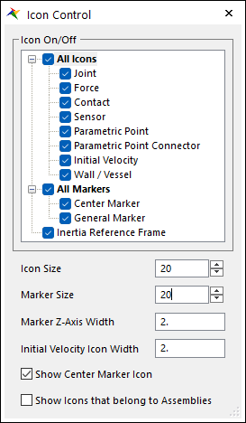
1.1.4.3. Adjusting the Icon and Marker Size

You are now going to change the icon and marker size to 20 pixels so you can view the model better.

1.1.4.3.1. To change the icon and marker size:

1. From Render Toolbar, click the Icon Control tool. The Icon Control dialog box appears.

2. Set Icon Size and Marker Size to 20.

3. Close the Icon Control dialog box (use the x in the upper right corner).

   

1.1.4.4. Creating Joints between the Bodies

1.1.4.4.1. To create fixed joint

You will fix Bracket to Ground to keep Bracket from moving

Tip

How to use Snap To Geometry in Select Toolbar

While creating a Joint, it is sometimes hard to find desired point with mouse navigation in working window. In this case, Snap To Geometry function will help you find the desired points.

• Snap To Grid: Find grid point

• Snap To Geometry: Find geometric point like Vertex, Center of Circle, etc.

• Snap To Node: Find node point of FE Body.

1. Disable the Snap To Geometry tool in Select Toolbar.

2. Click the Fixed Joint function from the Joint group in the Professional Tab.

3. Select Creation Method to Body, Body, Point.

4. Click entities and point using below information.

   • Body: Ground

   • Body: Bracket

   • Point: -150, 0, -50

   Fixed1 is created as shown at below.

   

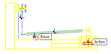
1.1.4.4.2. To create the revolute joint:

In this section, you will create the revolute joint between the grounded bracket and the crank.

1. From the Joint group in the Professional tab, click the Revolute Joint function.

2. Set the Creation Method to Body, Body, Point, Direction.

3. Click two bodies and two points using information below. (Point is center of rotation of Revolute Joint and Direction is direction of rotation axis)

   • Body: Bracket

   • Body: Crank

   • Point: -70, 0, 170

   • Direction: 1, 0, 0

     

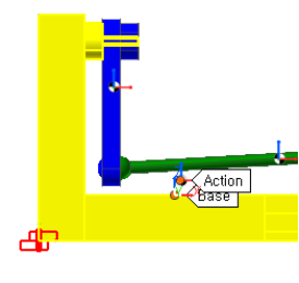
1.1.4.4.3. To create spherical joints

Now you will create the two spherical joints that connect between the crank and the connecting rod and between the connecting rod and the slider

1. From the Joint group in the Professional tab, click the Spherical Joint function.

2. Set the Creation Method to Body, Body, Point.

3. Click two bodies and one point.

   • Body: Crank

   • Body: Connecting_Rod

   • Point: -60, 0, 30

4. Repeat 1-3 steps using information below.

   • Body: Connecting_Rod

   • Body: Slider

   • Point: 290, 0, 50

     

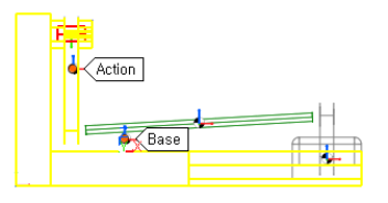
1.1.4.4.4. To create the translational joint:

Now you will create the translational joint between the slider and the grounded bracket.

1. From the Joint group in the Professional tab, click the Translational Joint function.

2. Set the Creation Method to Body, Body, Point, Direction.

3. Click two bodies and two points in the Working Window. (Point will be center of translation and Direction will be axis of translation)

   • Body: Bracket

   • Body: Slider

   • Point1: 300, 0, -20

   • Direction: 1, 0, 0

     

1.1.4.5. Creating a Motion on the Revolute Joint

Now you will define a motion on the revolute joint you just created.

1.1.4.5.1. To define a motion:

1. Display the Properties dialog box of RevJoint1. Click the Joint page and check the Include Motion box.

   

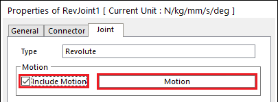
2. Click Motion.

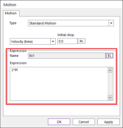
3. The Motion dialog box appears. Pull down on the second pull-down menu and set the motion type to Velocity (time).

   

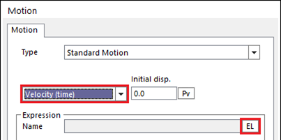
4. Click EL in the Motion dialog.

5. When the Expression List dialog box appears. Click Create.

   

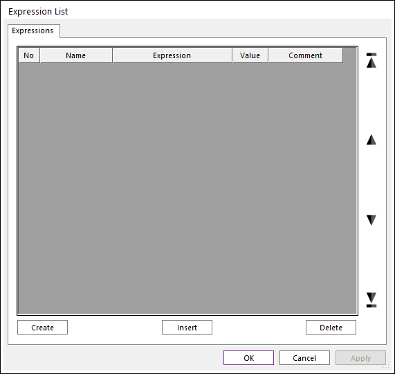
6. When the Expression dialog box appears. Input expression below.

   • 2*PI

     

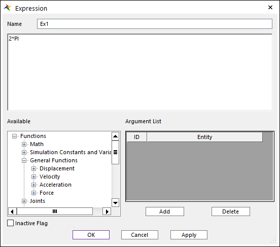
7. Click OK in Expression dialog.

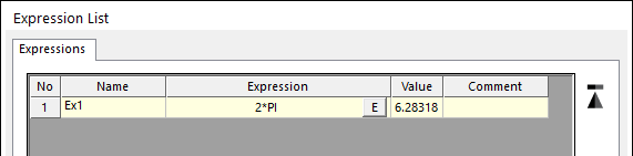
8. When the Expression List dialog box reappears, click Ex1 once to and OK.

   

9. In the Motion dialog box, check if Expression is displayed and click OK.

   

10. In the Joint dialog box, click OK.

1.1.5. Performing Analysis

1.1.5.1. Task Objective

In this chapter, you will run a simulation of the model you just created.

1.1.5.2. Estimated Time to Complete

5 minutes

1.1.5.3. Performing Dynamic/Kinematic Analysis

In this section, you will run a dynamic/kinematic analysis to view the effect of forces and motion on the model you just created.

1.1.5.3.1. To perform a dynamic/kinematic analysis:

1. From the Simulate Type group in the Analysis tab, click the Dynamic / Kinematic Analysis function. The Dynamic/Kinematic dialog box appears.

   

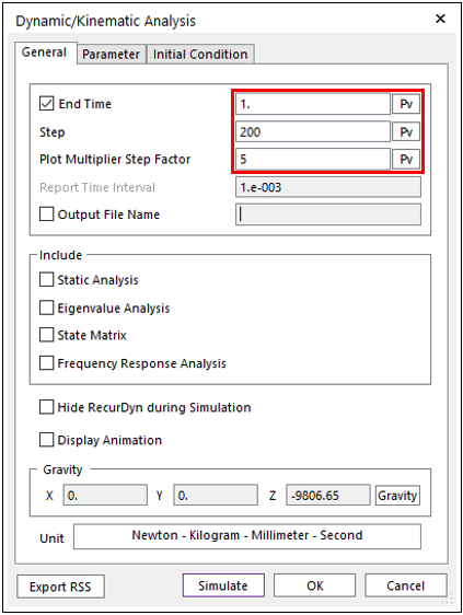
2. Define the end time of the simulation and the number of steps:

   • End Time: 1

   • Step: 200

   • Plot Multiplier Step Factor: 5

3. Click Simulate. RecurDyn calculates the motions and forces acting on the slider crank.

Tip

Meaning of Options in Simulate dialog box

Here is a quick list of the most commonly used options in the Dynamic/Kinematic dialog box:

• End Time: Defines the length of the Simulation Time.

• Step: Defines the number of animation frames to store throughout the simulation time.

• Plot Multiplier Step Factor: Defines the number of data points that are saved for plotting.

  The number of the plot data points that are stored is defined as: Step*Plot Multiplier Step Factor

1.1.6. Working with Animations

1.1.6.1. Task Objective

In this chapter, you will learn how to animate the motion of the model and how to create an AVI file of the animation for use in presentations. You will also learn how to trace the paths of points on the moving bodies.

1.1.6.2. Estimated Time to Complete

10 minutes

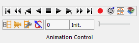
1.1.6.3. About the Animation Toolbar

You can animate your model after simulating. When you work with animations after loading the model in RecurDyn/Plot you can play the animations as you display the plots to more completely analyze the data. The Animation Toolbar from Animation Control group in the Analysis tab is shown below. Each of its tools are explained in the table below.

The tool	Does the following:
	Go to the first frame.
	Fast Reverse Play/Pause
	Go back one frame
	Reverse Play/Pause
	Stop
	Play/Pause
	Go forward one frame
	Fast Play/Pause
	Go to last frame.
	Record (must be stopped)
	Reload the last animation file
	Multi Animation
	Scenario output control
	Animation Scaling
	Select camera
	Animation control configuration
	Force display setting

1.1.6.4. Playing Animations

From the Animation Control group in the Analysis tab, click the Play function.

1.1.6.5. Saving the Animation Data as an AVI File

Now you will save the animation you just viewed as an AVI file so you could post it to the Web or play it in a PowerPoint presentation.

1.1.6.5.1. To save an animation as an AVI file:

1. From the Animation Control group in the Analysis tab, click the Record function. The Video Settings dialog box appears.

   

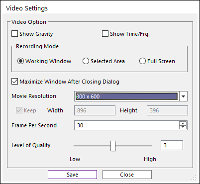
2. Define the size of the image in the AVI file by clicking on the combo box for the Movie Resolution field and selecting 800 x 600.

3. Click Save. The Save As dialog box appears.

4. Enter the file name and location for the AVI file.

5. Click Save.

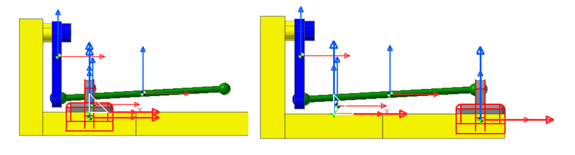
1.1.6.6. Tracing the Paths of Points on the Moving Bodies

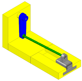
In the animation you saw that the motion of the crank, connection rod and slider bodies seem to move simply but it is not simple. Now you will trace out the path of a point on each body to better understand its motion. The point on each body will be defined by a marker. A marker is a coordinate system. It has an origin and an orientation. You will use some existing markers to trace some paths.

1.1.6.6.1. To trace the path of a point:

1. From the Post Tool group in the Analysis tab, click the Marker Trace function. The Marker Trace dialog box appears.

   

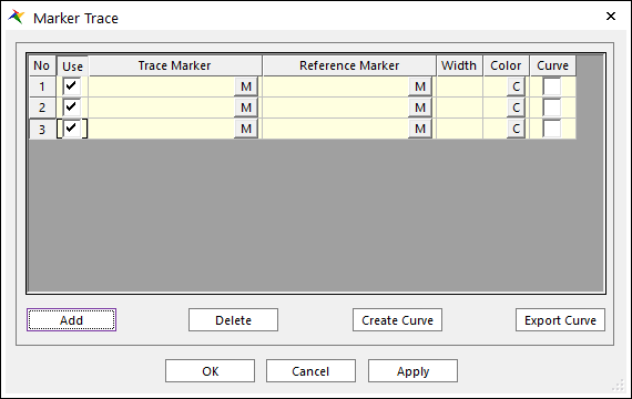
2. Click the Add button three times to create three lines in the dialog box.

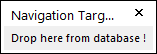
3. Each line will have a marker button. Click M for the first line. The Navigation Target Window will appear in the upper right of the Working window.

   

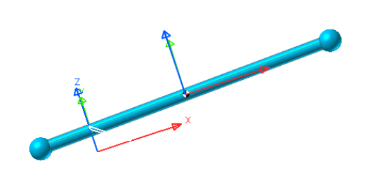
4. Expand the Crank, Connecting Rod, and Slider Body names in the Database window. Expand the Markers headings for the Crank, Connecting_Rod, and Slider Bodies. The Database Window should appear as shown at below.

   

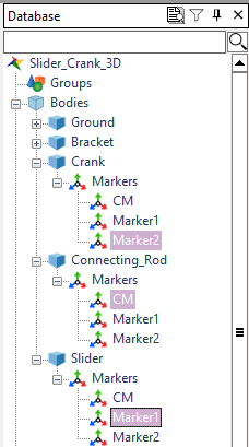
5. Select the Marker2 name under the Crank body and drag it to the Navigation Target Window. You should see the name Crank.Marker2 appears in the first row of the Trace Marker column.

6. Click on the Marker button for the second line.

7. Select the CM name under the Connecting_Rod body and drag it to the Navigation Target Window. You should see the name Connecting_Rod.CM appears in the second row of the Trace Marker column.

8. Click on the Marker button for the third line.

9. Select the Marker1 name under the Slider body and drag it to the Navigation Target Window. You should see the name Slider.Marker1 appears in the third row of the Trace Marker column.

   

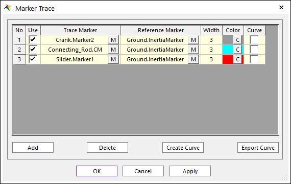
10. Set the Width in all three rows to 3.

11. Set the Color in the first row to light Gray by clicking C and selecting the color in the second row and the second column of the palette.

12. Set the Color in the second row to cyan by clicking C and selecting the Turquoise cell.

13. Set the Color in the third row to red by clicking C and selecting the Red cell. The Marker Trace dialog box should appear as in the figure.

14. Click OK to close the Marker Trace dialog box.

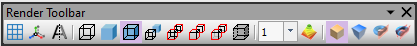
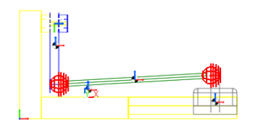
15. Play the animation again by clicking on the play button. You should see the three traces as shown in the figure.

    

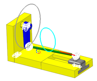
The traces suggest the type of motion that each body is experiencing.

• The trace of the slider is the red line, suggesting motion in a single degree of freedom.

• The trace of the crank is a circle, suggesting a rotational motion with translations in two directions.

• The trace of the connecting rod is a slanted circle, suggesting that the connecting rod is undergoing both a rotational motion and a translational motion. The CM marker in the Connecting Rod is translating in all three degrees of freedom.

Tip

How to use the Animation control configuration

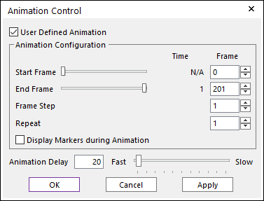
There are several configuration settings for animations that you can set when you select the Animation Configuration Tool function, from the Animation Control in the Analysis tab.

• Start Frame and End Frame: Defines the start frame and the end frame of an animation.

• Frame Step: Increment frame of an animation.

• Repeat: Defines the number of times to replay the animation.

• Display Markers during Animation: If you check this option, you can see the markers during an animation.

  

1.1.7. Plotting

1.1.7.1. Task Objective

In this chapter, you will plot the analysis data that RecurDyn calculated in the dynamic/kinematic simulation you ran in the previous chapter. You will plot the motion of the slider body, using RecurDyn/Plot, a powerful post-processing tool, which is built into RecurDyn. It lets you plot and animate the results of simulations.

1.1.7.2. Estimated Time to Complete

5 minutes

1.1.7.3. Creating a Plot

In this section, you will start RecurDyn/Plot and view a plot of the motion of the slider.

1.1.7.3.1. To start RecurDyn/Plot and plot the motion of the slider body:

1. From the Plot group in the Analysis tab, click the Plot Result function. The Plotting window appears with all the tools and data you need.

   

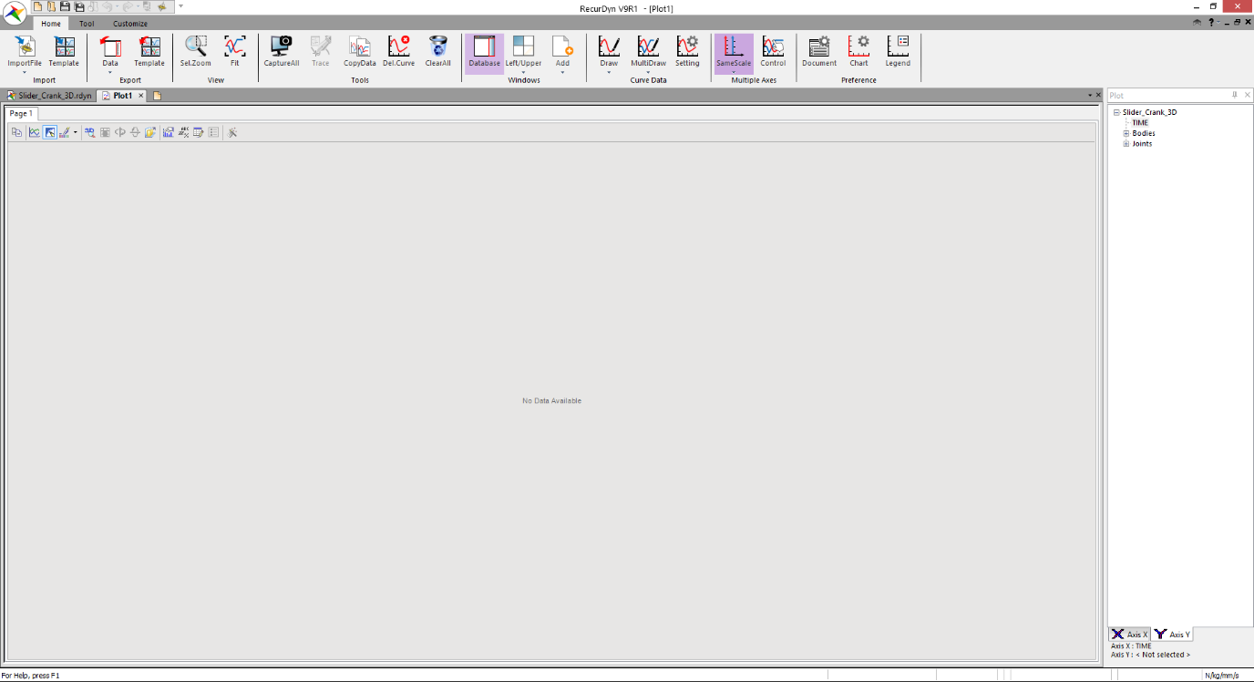
2. In the Plot Database Window, expand the Bodies heading, expand the Crank heading

3. Right-click on Pos_TX. Pos_TX is an abbreviation for Position in Translation along the X direction.

4. Select Draw from the pop-up menu that appears.

   

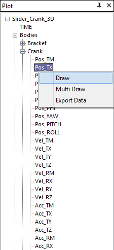
5. Now double-click on Pos_TY and Pos_TZ. You can see that double-clicking has the same effect as Steps 3 and 4. The plot should appear as in the figure.

   

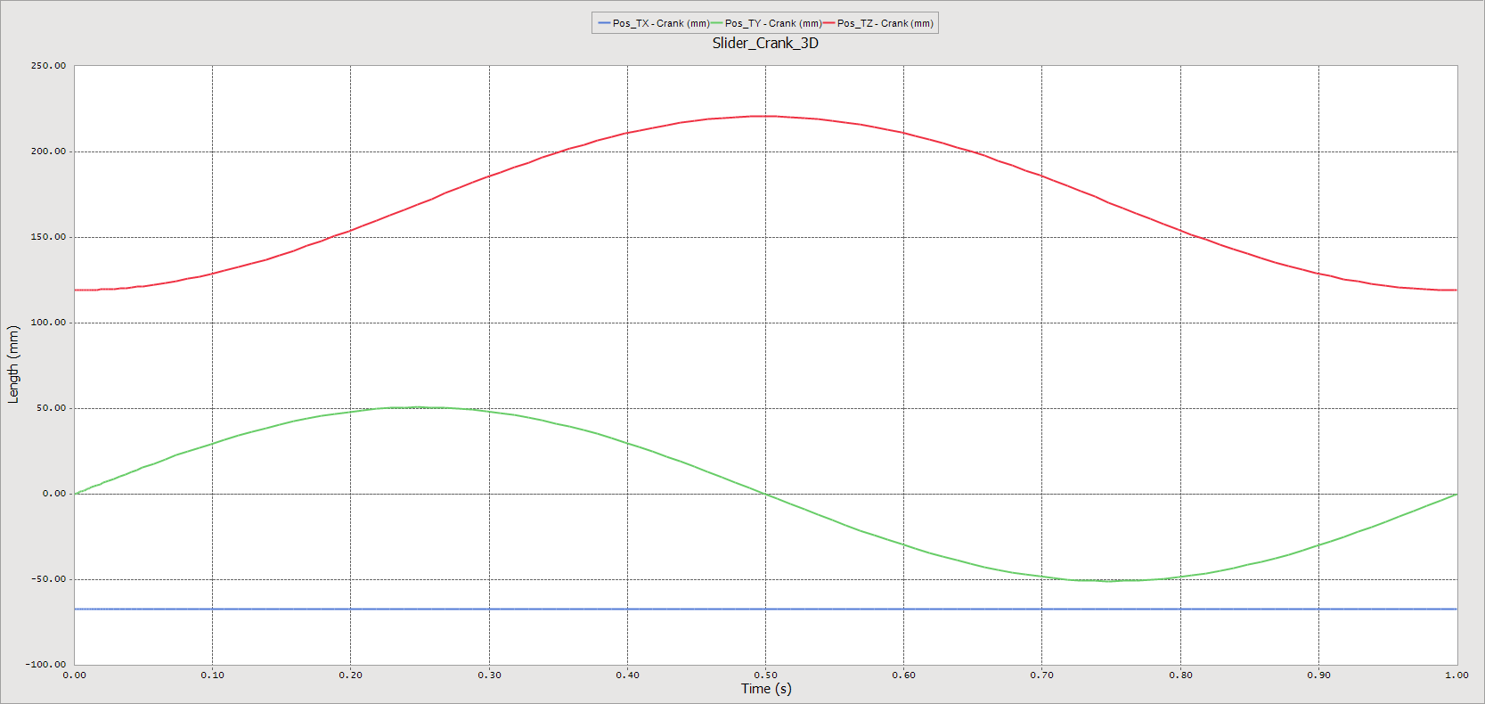
   Note that the plot gives us the same feedback as the Trace Curve for the Crank body (presented in the previous chapter), which is that the motion of the Crank included translations in two directions. There is no translation in the Z direction.

1.1.7.4. Plotting in Multiple Panes

In this section, you will learn how to use multiple panes in the Plotting Window to understand your model behavior more completely.

1.1.7.4.1. To switch the Plotting Window to display multiple panes:

1. From the Windows group in the Home tab, click the Show All Windows function. You should now see four plotting areas within the Plot Window.

2. Set the upper-right pane to be the active pane by clicking on any point within it.

3. In the Plot Database Window, expand the Connecting_Rod heading under the Bodies heading

4. Double-click on Pos_TX, then Pos_TY, then Pos_TZ as you did with the previous plot.

5. Set the lower-left pane to be the active pane by clicking on any point within it.

6. In the Plot Database Window, expand the Slider heading under the Bodies heading.

   

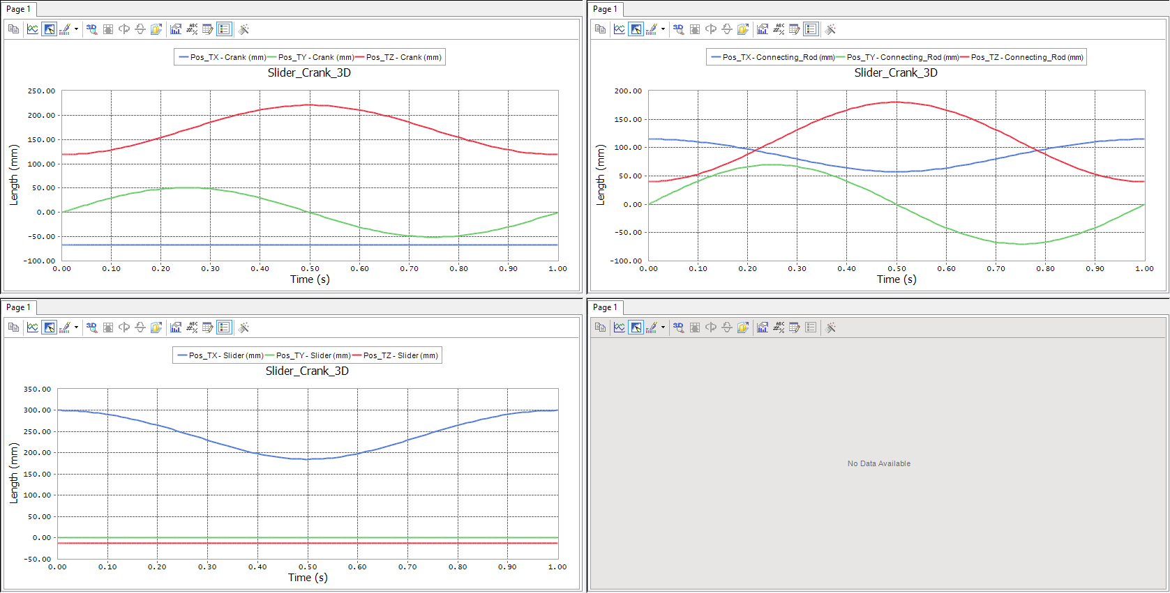
7. Double-click on Pos_TX, then Pos_TY, then Pos_TZ as you did with the previous plot. The plot should appear as in the figure. The curves in the plot for the slider body show us that the body is moving in one translational degree of freedom. The curves in the plot for the connecting rod body show us that the body is moving in all three translational degree of freedom.

1.1.7.5. Loading an Animation

In this section, you will load an animation into one of the pane in the Plotting Window in order to display a coordinated view of output values and the motion of the mechanical system. Note that an AVI file of the combined plots and animation can be created by following the same steps that were outlined in the previous chapter.

1.1.7.5.1. To load an animation in a pane of the Plotting Window:

1. Set the lower-right pane to be the active pane by clicking on any point within it.

2. From the Animation group in the Tool tab, click the Load Animation function. The following alert box appears:

   

3. Click Yes and the animation will be loaded in the lower-right pane.

4. Change to the XZ plane.

5. Type F key to fit the model within the pane.

6. Type R key and drag the cursor in the pane to rotate the model into a better viewing position. Repeat the fit command as needed. The Plotting Window should appear to be similar to the figure shown on the cover of this tutorial.

7. Play the animation by clicking the Play function.

Tip

If you want to restore Animation section to Plot section, use the Load Plot function from the Animation group in the Tool tab.