7.2. Plasticity Bending Machine Tutorial (FFlex)
7.2.1. Overview
A bending machine bends metal plates by holding them between its upper and lower frames and applying pressure to the plate. Different bending frames bend plates into different angles and shapes.
The shapes of the frames determine how a bending machine deforms the metal plate. The force applied by the bending machine creates a stress that exceeds the yield stress of the plate, so the plate is permanently deformed (plastic deformation). Therefore, to understand the plastic behavior of a metal plate, you must perform a plastic analysis rather than an elastic analysis.
To perform a plastic analysis, you must give a flexible body modeled in RecurDyn with plastic properties instead of elastic properties and simulate the behavior of the flexible body.
In this tutorial, you will learn how to assign plastic properties to a dynamic model composed of flexible bodies and perform a plastic analysis. You will also learn about the characteristics of a plastic analysis by comparing the results of the analysis to the results obtained using an elastic material.
7.2.1.1. Task Objective
This tutorial covers the following topics:
Elastic analysis of the behavior of a flexible body
Requirements for performing a plastic analysis
How to apply plastic properties to an analysis model and the characteristics of plastic analysis
How to analyze the results of a plastic analysis
Differences between an elastic analysis and a plastic analysis
7.2.1.2. Prerequisites
This tutorial is intended for users who have completed the Basic and FFlex/RFlex tutorials provided with RecurDyn. If you have not completed these tutorials, then you should complete them before proceeding with this tutorial. In addition, this tutorial requires a basic understanding of dynamics and the finite element method.
7.2.1.3. Procedure
The following table outlines the tasks involved in this tutorial and their duration.
Procedure |
Time (minutes) |
Opening the Initial Model |
5 |
Generating a FFlex Body |
20 |
Performing an Elastic Analysis |
10 |
Performing a Plastic Analysis |
5 |
Analyzing and Reviewing the Results |
10 |
Total |
65 |
7.2.1.4. Estimated Time to Complete
65 minutes
7.2.2. Opening the Initial Model
7.2.2.1. Task Objective
Open the initial model, perform a simulation, and observe the behavior of the bending machine.
7.2.2.2. Estimated Time to Complete
5 minutes
7.2.2.3. Opening the RecurDyn Model
7.2.2.3.1. To run RecurDyn and open the initial model:
On the Desktop, double-click the RecurDyn icon to open RecurDyn. When the Start RecurDyn dialog window appears, close it.
In the File menu, click the Open function.
- Navigate to the Plasticity tutorial folder and select Plasticity_Bending_Machine_Start.rdyn.(File path: <InstallDir>\Help\Tutorial\Flexible\FFlex\Plasticity_Bending_Machine)
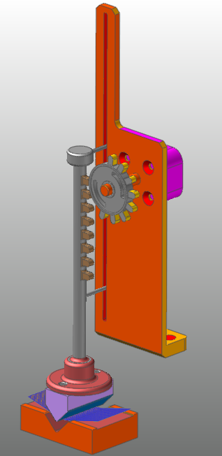
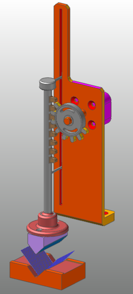
Click Open to open the model shown in the following figure.
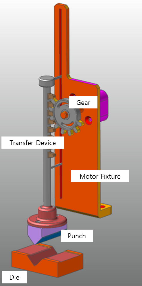
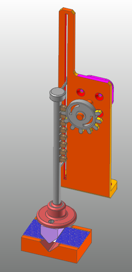
The following explains the configuration of the model.
The figure on the above shows a type of bending machine. The motor turns the gear to raise the transfer device. When the transfer device reaches the final tooth on the gear, the transfer device drops to strike the metal plate (placed on the die) with the punch.
The figure on the above does not include the metal plate. Later in this tutorial, you will learn how to model a metal plate using a flexible body. To do so, you model a metal plate with plastic properties on top of the die. The energy of the falling punch and transfer device is applied to the metal plate through an impact to deform it.
When the punch hits it, the metal plate deforms in the shape of the die. The teeth on the gear then engages the teeth on the transfer device to raise the punch again.
The model used in this tutorial consists of a die, punch, transfer device, motor fixture, and gear. You will model the metal plate later in the tutorial.
7.2.2.3.2. To save the model:
In the File menu, click the Save As function.
(You cannot perform the simulation if the model is in the tutorial path, so you must save the model in a different path.)
7.2.2.4. Simulating the Initial Suspension Model
This section teaches you how to conduct an initial simulation using the model in order to understand its behavior.
7.2.2.4.1. To perform the initial simulation:
On the Analysis tab, in the Simulation Type group, click the Dynamic/Kinematic Analysis function. The Dynamic/Kinematic Analysis dialog window appears.
Set the End Time and Step fields as follows:
End Time: 2
Step: 200
Plot Multiplier Step Factor: 1
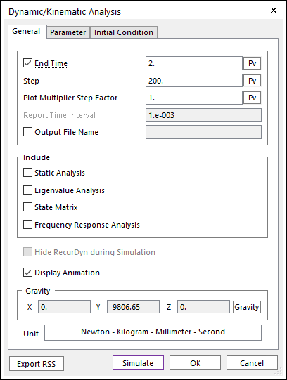
Click Simulate.
7.2.2.5. Viewing the Result
7.2.2.5.1. To view the results:
On the Analysis tab, in the Animation Control group, click Play.
In the work pane, the motor turns the gear to raise the transfer device. After the transfer device passes the final tooth on the gear, the punch falls and strikes the die. The gear then engages the transfer device again to raise it.
7.2.3. Generating a FFlex Body
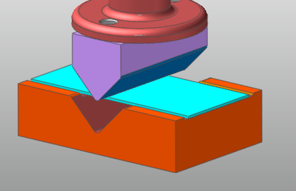
As mentioned previously, the current RecurDyn model does not include the metal plate model needed to perform plastic analysis. Therefore, to create the flexible body for the metal plate, you must first create a rigid body using the box geometry provided in RecurDyn. Then, you can transform the rigid body into a flexible body using the Mesher. You must also define the contact points between the metal plate and die as well as the metal plate and punch.
7.2.3.1. Task Objectives
This task teaches you how to replace the newly created rigid body with a flexible body using the Mesher provided in RecurDyn/FFlex (Full Flex).
7.2.3.2. Estimated Time to Complete
20 minutes
7.2.3.3. Creating the Box Geometry
On the Professional tab, in the Body group, click the Box function.
In the Modeling Options dropdown menu, select Point, Point and then type the following values in the Input Window Toolbar.
-75, 0, 35 (Press Enter after typing the values.)
75, -2, -35 (Press Enter after typing the values.)
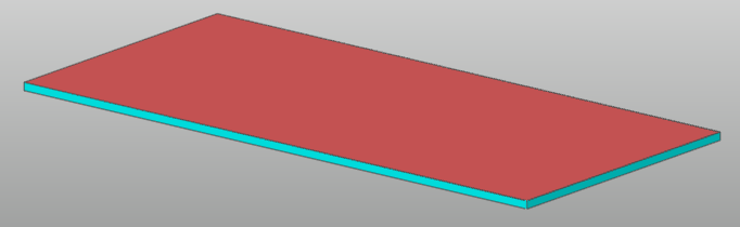
After you enter the values, the box geometry (shown below) appears.
In the Database Window, change the name of Body1 to Plate.
7.2.3.4. Creating the Box Mesh
In Assembly mode, right-click the work pane to display the context menu and click Mesh.
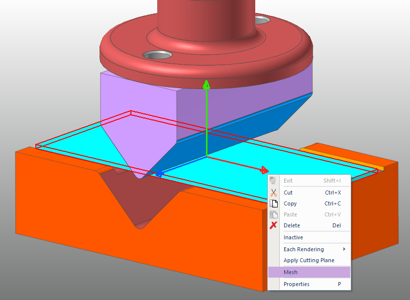
Mesh mode displays only the plate body, as shown below.
On the Geometry tab, in the Surface group, click the Face Surface functions.
Select Box1 to open the FaceSurf Operation dialog window. With the FaceSurf Operation dialog window open, select Box1.Face4 on top of the box.
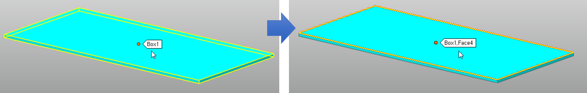
When Face4 appears in the dialog window (shown below), click OK to create FaceSurface1.
On the Mesher tab, click the Auto Mesh function to open the Mesh dialog window.
In the Mesh dialog window, perform the following:
In the Target Geometry option, Click Gr then select FaceSurface1.
In the Mesh Type dropdown menu, select Shell4(Quad4).
In the Mesh Option group, set both the Max Element Size and Min Element Size to 3.
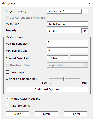
Click Mesh.
Click Cancel.
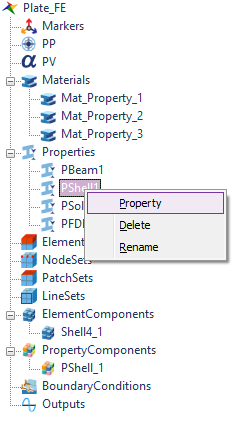
In the Database Window, under the newly created Plate, right-click PShell1, and then click Properties in the context menu to open the Property dialog window.
In the Property dialog window, click … to the right of No. 2 PShell1. When the Property Shell dialog window appears, change the Thickness from 10 to 0.5, and then click Close.
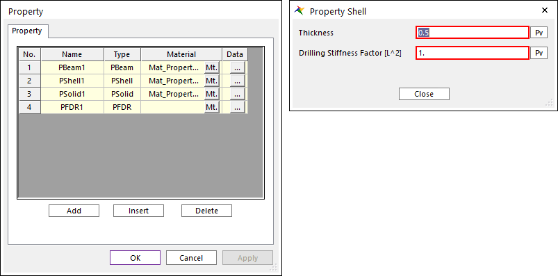
In the Property dialog window, click Mt. to the right of No. 2 PShell1. The Material dialog window appears (shown below).
In the Material dialog window, click … to the right of No. 2, and then change the following settings:
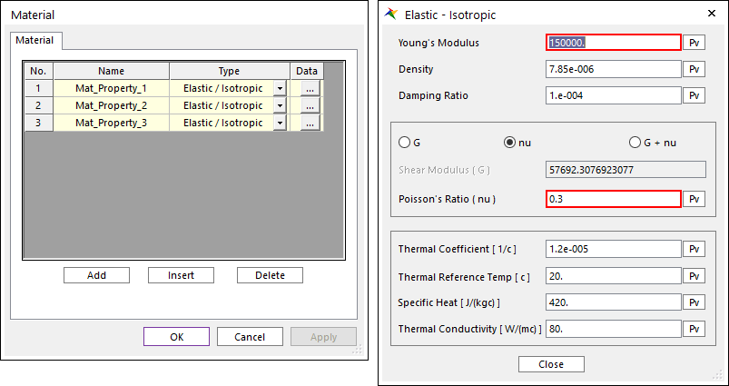
Change the Young’s Modulus value from 200,000 to 150,000.
Select nu, and then change Poisson’s Ratio to 0.3. Then, click Close.
Click OK twice to close all open dialog windows.
In the FFlex Edit group, click the Boundary Condition function. When the dialog window appears, click Add/Remove.
Press Shift key and Z key at the same time to change the working plane to the ZX plane. Then, click and drag the mouse to select the nodes located at the center of the plane.
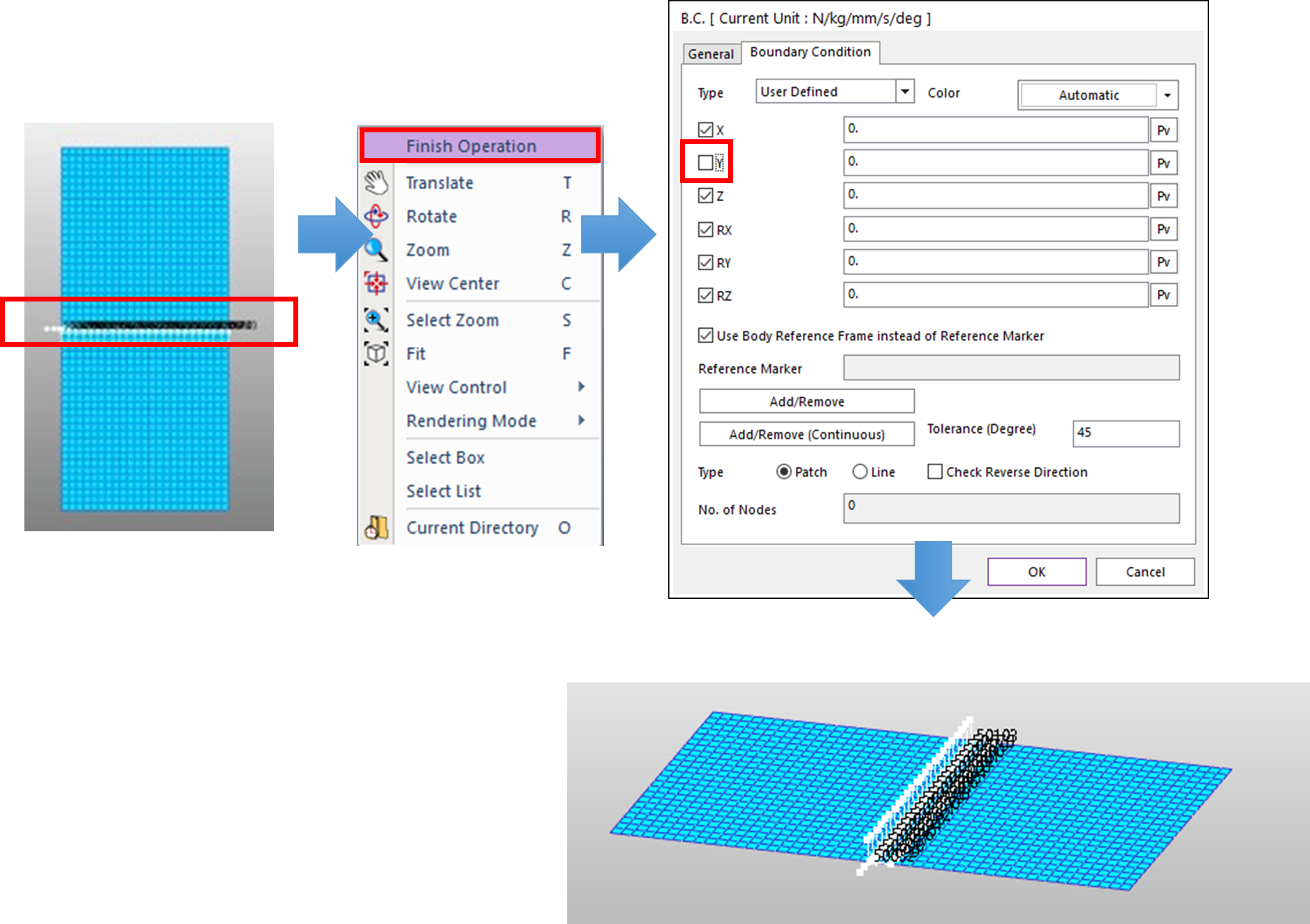
Once you select the nodes on which to apply the boundary condition, right-click the screen and select Finish Operation from the context menu. (For your information, the ID of the leftmost node is 50103.)
When the Property dialog window appears again, clear the Y checkbox, as shown below. Click OK to see the new boundary conditions created on the screen.
Tip
If you don’t see the node IDs, click Show IDs in the Flexible toolbar.
Use one of the following methods to return to a higher menu:
Right-click the working pane to display the context menu, and then click Exit.
On the Mesher tab, in the Exit group, click the Exit function.
Tip
Setting the boundary conditions for the FFlex Body as such removes the constraint on the Y axis (the direction in which the punch travels) but maintains the constraint for the remaining DOFs in the center of the plate, where deformation is not expected to occur, in order to increase the speed of analysis.
7.2.4. Performing Elastic Analysis
7.2.4.1. Task Objectives
In this chapter, you will learn how to conduct dynamic modeling and analysis on a FFlex Body and check the results of the analysis.
7.2.4.2. Estimated Time to Complete
10 minutes
7.2.4.3. Performing Dynamic Modeling
7.2.4.3.1. To create a patch set:
Double-click the Plate body to enter Body Edit Mode.
On the FFlex Edit tab, in the Set group, click the Patch Set function.
When the Patch Set dialog window appears, click Add/Remove. Then, in the Working Window, click and drag the mouse to select the whole body.
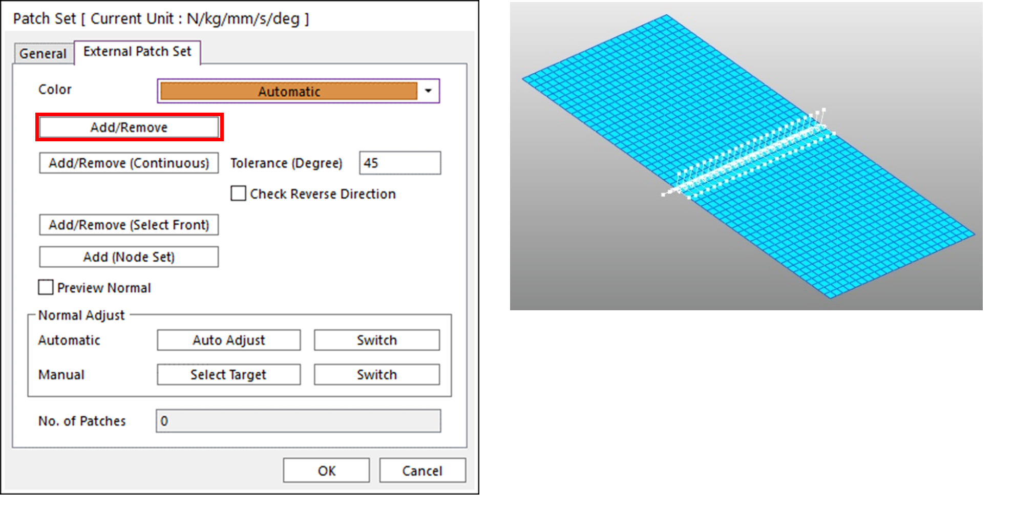
Right-click the Working Window to display the context menu, and then click Finish Operation.
In the Patch Set dialog window, click OK.
Confirm that SetPatch1 appears in the Database Window.
Click the Patch Set function again and repeat steps 3 and 4 to create another patch set. In the Patch Set dialog window, select the Preview Normal checkbox, as shown below. Then, in the Automatic row of the Normal Adjust group, click Switch. (This process creates two patch sets to define the contacts on both sides of the shell.)
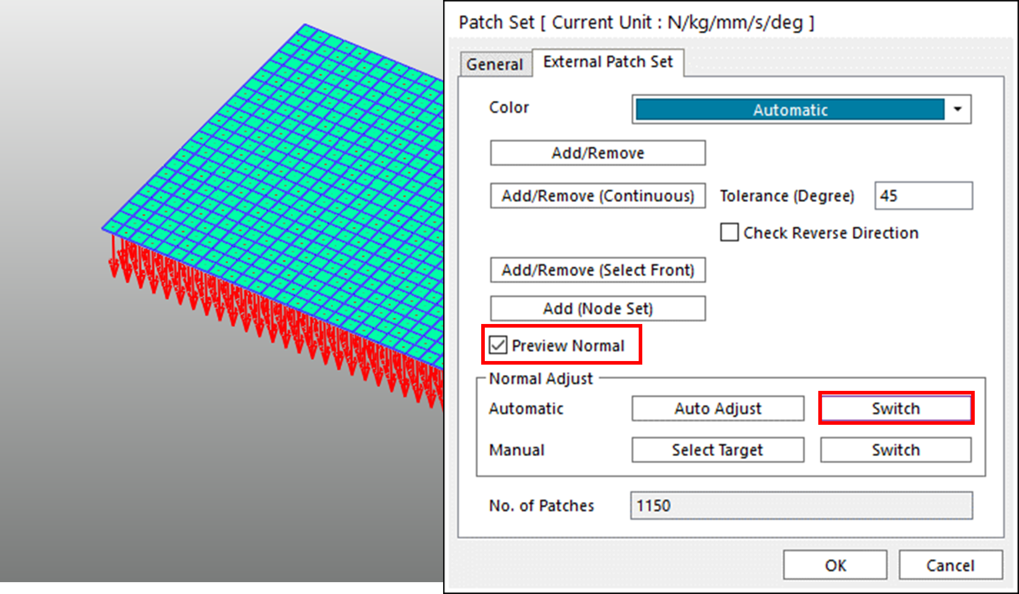
In the Patch Set dialog window, click OK.
Confirm that SetPatch2 appears in the Database Window.
On the FFlex Edit tab, in the Exit group, click the Exit function to return to a higher menu.
7.2.4.3.2. To create a contact:
On the Professional tab, in the Contact group, click the Geo Surface Contact function. Then, in the Modeling Option dropdown menu, select Surface(PatchSet), Surface(PatchSet), as shown below.
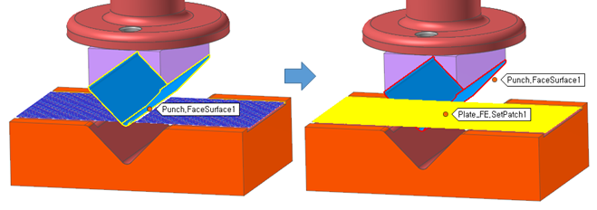
Select Punch.FaceSurface1, which will be designated as the base body for the geo surface contact, and Plate.SetPatch1, which will be designated as the action body. Confirm that GeoSurContact3 is created in the Database Window.
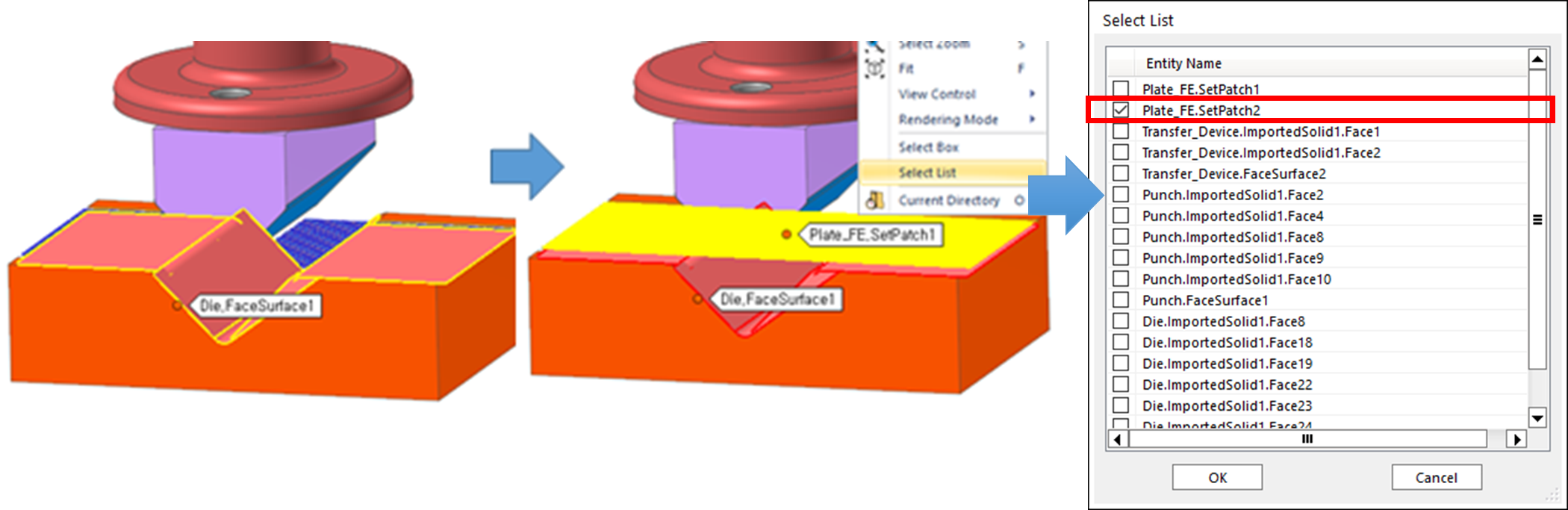
Click the Geo Surface Contact function again. Then, select the areas that will become the base and action bodies for the geo surface contact, as shown below, to create GeoSurfaceContact4.
For the base body, select Die.FaceSurface1.
For the action body, it is difficult to select Plate.SetPatch2 in the work pane. So, right-click the screen to display the context menu, and then click Select List. When the Select List dialog window appears, select the Plate.SetPatch2 checkbox.
To see if the geo surface contacts are set properly, right-click GeoSurContact4 to open the Properties dialog window.
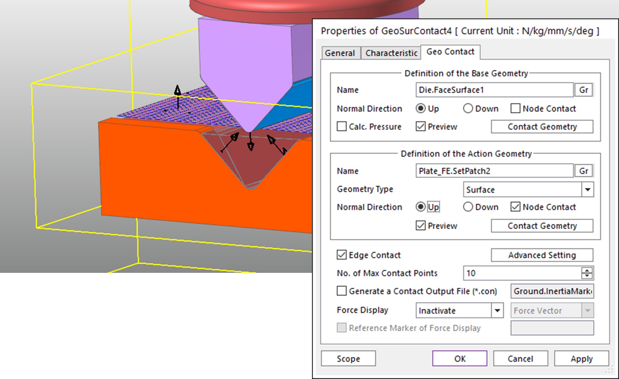
In the Definition of the Action Geometry group, click Contact Geometry. When the Surface Patch dialog window appears, change the Bounding Buffer Length to 25.
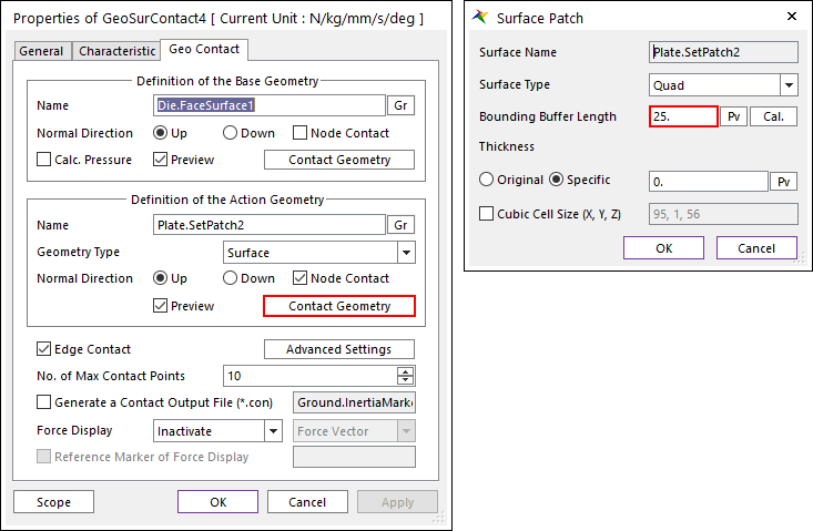
Perform the same process for GeoSurContact3, but leave the Normal Direction set to Up. Only change the Bounding Buffer Length for Plate.SetPatch1 to 25.
7.2.4.4. Performing Elastic Analysis
In this procedure, you will learn how to perform a simulation on the FFlex body created earlier and the contacts defined for elastic analysis.
7.2.4.4.1. To run the simulation:
On the Analysis tab, in the Simulation Type group, click the Dynamic/Kinematic Analysis function. The Dynamic/Kinematic Analysis dialog window appears.
Set the End Time and Step fields as follows:
End Time: 2
Step: 200
Plot Multiplier Step Factor: 1
Click Simulate.
7.2.4.4.2. To view the results:
On the Analysis tab, in the Animation Control group, click the Play function.
Unlike the transfer device in previous simulation, in which the punch came into direct contact with the die, the transfer device in this simulation behaves differently because the contact occurs between the Plate flexible body and the punch and die.
The Plate flexible body acts as a spring when the punch falls on it, and the transfer device rebound upwards. This phenomenon does not occur in real life. The reason why this phenomenon occurs is because the Plate flexible body has only elasticity, not plasticity. Therefore, even though a large amount of deformation occurs, the flexible body return to its original state, springing the transfer device upwards.
Due to this spring effect, the transfer device is raised without the help of the gear and must remain aloft until the final gear tooth.
Therefore, to realistically simulate the deformation of a metal plate and the operation of a transfer device, you must add plasticity to the flexible body and perform plastic analysis rather than elastic analysis.
7.2.4.4.3. To check the contour results:
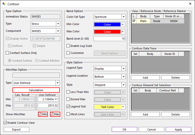
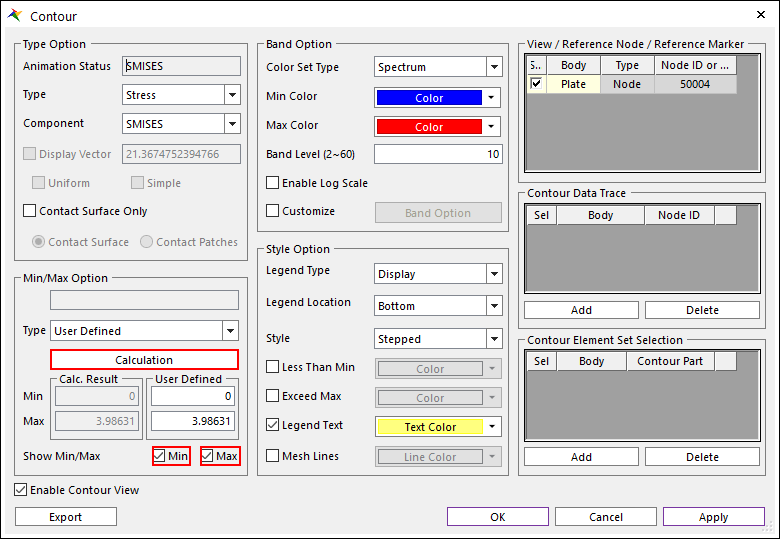
On the Flexible tab, in the FFlex group, click the Contour function. The Contour dialog window appears.
In the Contour dialog window, perform the following:
Click Calculation in the middle of the dialog window.
Select Min and Max checkboxes of Show Min/Max.
Click OK to see the results.
On the Analysis tab, in the Animation Control group, click Play.
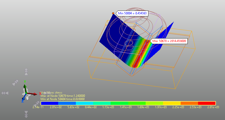
To see the contour result for Plate, as shown below, click the Wireframe tool in the Render Toolbar and run the animation.
At 1.24 seconds, you can see that the Maximum Von-Mises Stress is approximately 2814 MPa.
7.2.5. Performing Plastic Analysis
7.2.5.1. Task Objectives
In this chapter, you will learn how to apply plastic properties to an FFlex body and check the results after performing plastic analysis.
7.2.5.2. Estimated Time to Complete
20 minutes
7.2.5.3. Performing Plastic Modeling (1)
7.2.5.3.1. To create a plastic material:
Double-click the Plate body to enter Body Edit Mode.
In the Database Window, right-click Plate, and then click Edit in the context menu. Then, double-click Mat_Property_2 to open the Material Property dialog window, as shown below.
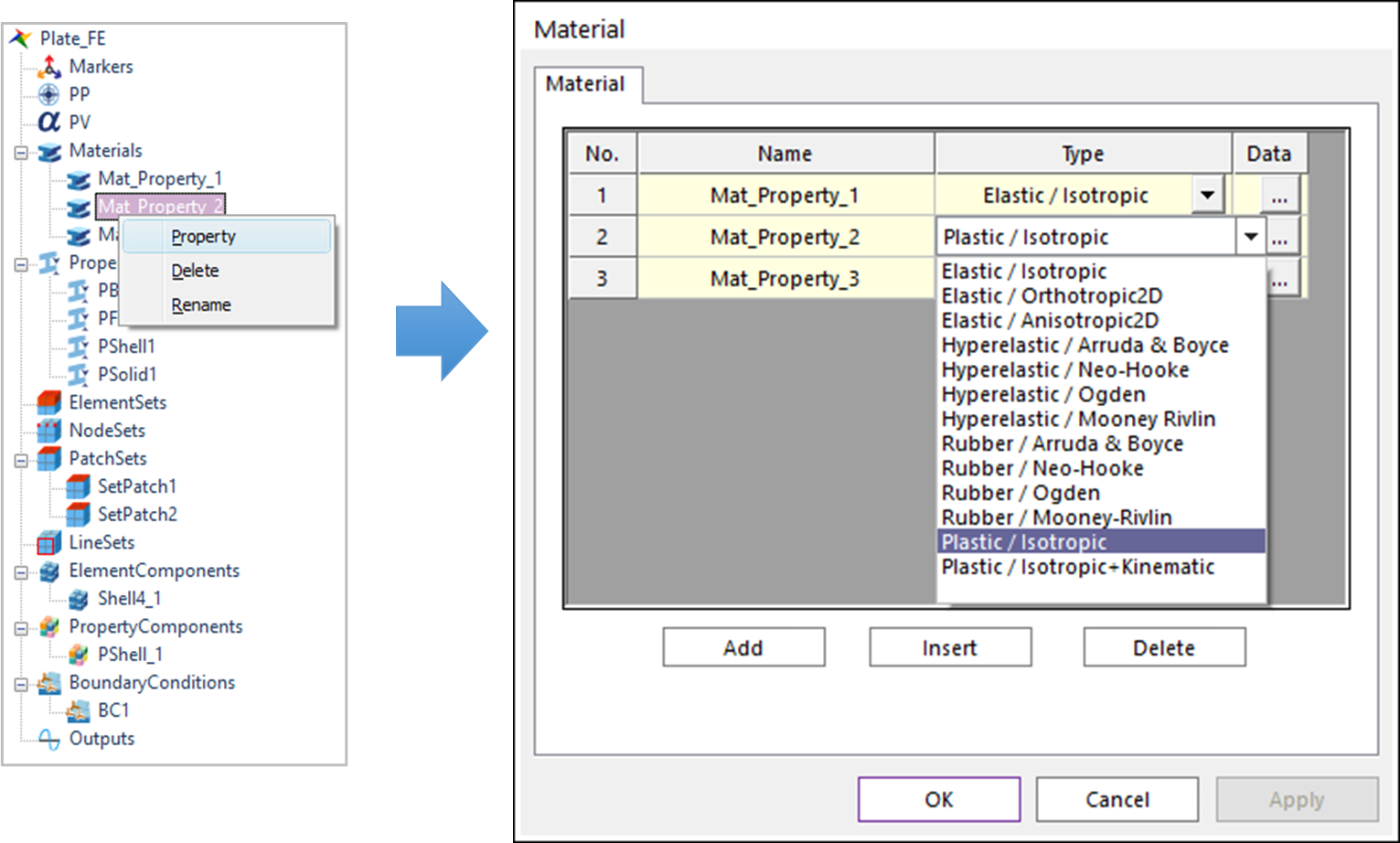
In the Material dialog window, select Plastic/Isotropic in the dropdown menu to the right of Mat_Property_2 (No. 2). Then, click the … button to display the Plastic - Isotropic dialog window.
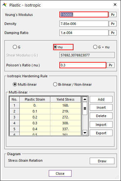
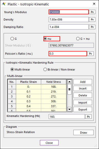
In the Plastic - Isotropic dialog window, perform the following:
Change the Young’s Modulus value from 200,000 to 150,000.
Select the Nu radio button and change Poisson’s Ratio to 0.3.
In the Multi-linear group, click Add to add a new row. Then, type in the Plastic Strain and Yield Stress values shown in the following table.
No.
Plastic Strain
Yield Stress
1
0
168
2
0.1
219
3
0.2
272
4
0.3
308
5
0.4
337
6
0.5
361
7
0.6
382
8
0.7
401
9
0.8
418
10
0.9
434
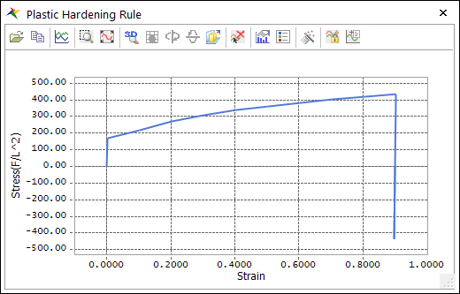
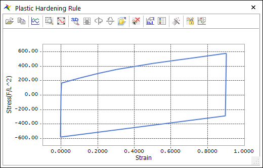
To ensure that the values entered in the previous step are correct, in the Diagram group, click Draw to the right of the Stress-Strain Relation menu and ensure that the graph resembles the graph shown below.
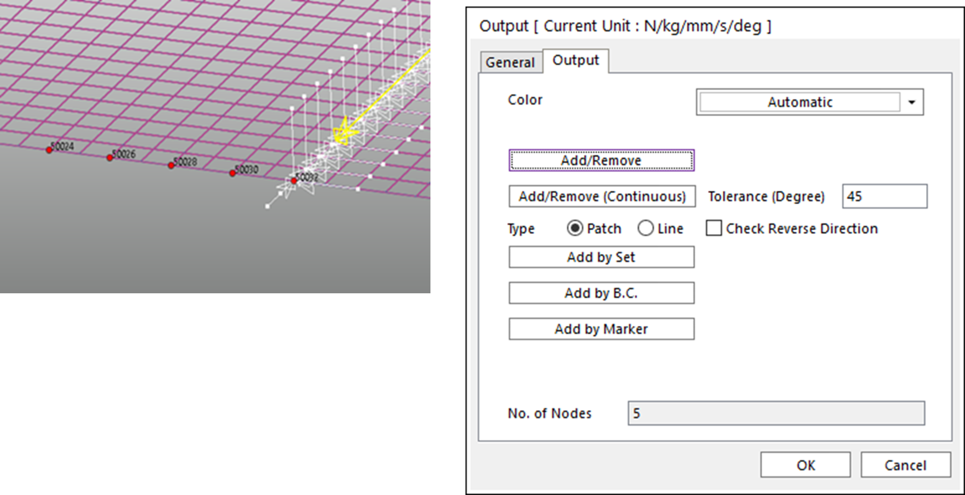
In the FFlex Edit group, click the Output function. When the Output Current Unit dialog window appears, click Add/Remove.
Hold down the Shift key and click the five nodes (50032, 50030, 50028, 50026, and 50024), as shown below.
After selecting the nodes, right-click the work pane to display the context menu, and then click Finish Operation.
In the Outputs dialog window, click OK.
On the FFlex Edit tab, in the Exit group, click the Exit function to return to a higher menu.
In the File menu, click the Save As function. Then, save the model as Plasticity_Bending_Machine_Isotropic.rdyn.
7.2.5.4. Performing Plastic Analysis (1)
To see the results of the plastic analysis for the plastic material, you must run the simulation.
7.2.5.4.1. To run the simulation:
On the Analysis tab, in the Simulation Type group, click the Dynamic/Kinematic Analysis function. The Dynamic/Kinematic Analysis dialog window appears.
Set the End Time and Step fields as follows:
End Time: 2
Step: 200
Plot Multiplier Step Factor: 1
Output File Name: Isotropic_Plasticity
Click Simulate.
7.2.5.4.2. To view the results:
On the Analysis tab, in the Animation Control group, click Play.
Unlike the results of the elastic analysis, the metal plate in the plastic analysis remains in the V-shape of the die after the punch strikes.
In addition, the spring effect from the elasticity has disappeared, so the transfer device does not rebound. Because of this, the transfer device is raised again when the gear engages the teeth on the transfer device again, and the process is repeated.
7.2.5.4.3. To check the contour results:
On the Flexible tab, in the FFlex group, click the Contour function to display the Contour dialog window.
In the Contour dialog window, perform the following:
Click Calculation in the middle of the dialog window.
Select the Min and Max checkboxes of Show Min/Max.
Click OK to see the results.
On the Analysis tab, in the Animation Control group, click the Play function.
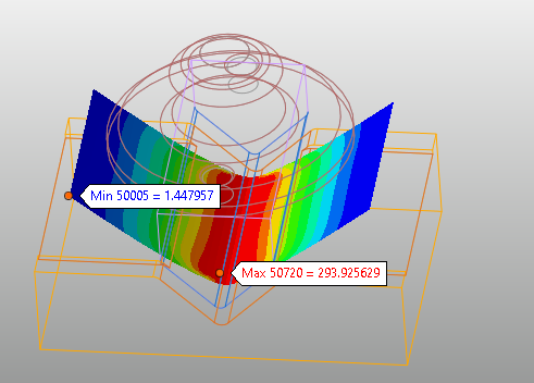
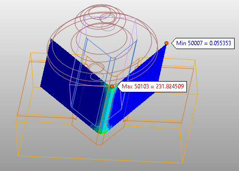
To see the contour result for Plate, as shown below, click the Wireframe tool in the Render Toolbar and run the animation.
You can see that, at 1.23 seconds, the Maximum Von-Mises Stress is approximately 293.93 MPa. After 1.52 seconds, approximately 231.82 MPa of residual stress remains.
7.2.5.5. Performing Plastic Modeling (2)
7.2.5.5.1. To create a plastic material:
Double-click the Plate body to enter Body Edit Mode.
In the Database Window, right-click Plate, and then select Edit in the context menu. Then, double-click Mat_Property_2 to open the Material Property dialog window, as shown below.
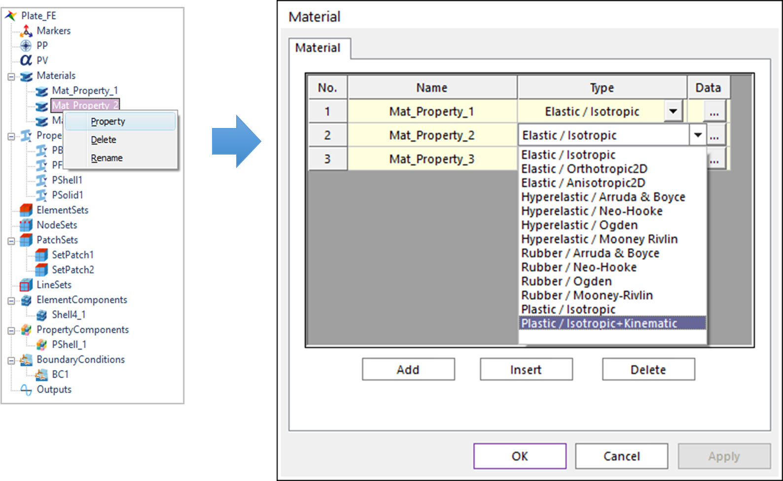
In the Material dialog window, select Plastic/Isotropic + Kinematic in the dropdown menu to the right of Mat_Property_2 (No. 2). Then, click the … button to display the Plastic - Isotropic-Kinematic dialog window.
In the Plastic - Isotropic-Kinematic dialog window, perform the following: (If you carried out the procedure described in Performing Plastic Modeling (1), you don’t need to change the Young’s Modulus and Nu options.)
Change the Young’s Modulus value from 200,000 to 150,000.
Select the Nu radio button and change Poisson’s Ratio to 0.3.
In the Multi-linear group, click Add to add a new row. Then, type in the Plastic Strain and Yield Stress values shown in the upper table.
No.
Plastic Strain
Yield Stress
1
0
168
2
0.1
219
3
0.2
272
4
0.3
308
5
0.4
337
6
0.5
361
7
0.6
382
8
0.7
401
9
0.8
418
10
0.9
434
In the Kinematic Hardening (Hk) field, type 160.
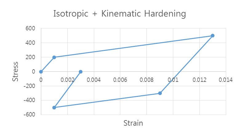
To ensure that the values entered in the previous step are correct, in the Diagram group, click Draw to the right of the Stress-Strain Relation menu. Ensure that the graph resembles the one shown below.
On the FFlex Edit tab, in the Exit group, click the Exit function to return to a higher menu.
In the File menu, click the Save As function, and save the model as Plasticity_Bending_Machine_Isotropic_Kinematic.rdyn.
7.2.5.6. Performing Plastic Analysis (2)
To see the results of the plastic analysis for the plastic material, you must run another simulation.
7.2.5.6.1. To run the simulation:
On the Analysis tab, in the Simulation Type group, click the Dynamic/Kinematic Analysis function. The Dynamic/Kinematic Analysis dialog window appears.
Set the End Time and Step fields as follows:
End Time: 2
Step: 200
Plot Multiplier Step Factor: 1
Output File Name: Isotropic_Kinematic_Plasticity
Click Simulate.
7.2.5.6.2. To view the results:
On the Analysis tab, in the Animation Control group, click the Play function.
Just like the results of Performing Plastic Analysis (1), the metal plate in this simulation maintains the V shape of the die after the punch strikes it.
Because of this, the transfer device is raised again when the gear engages the teeth on the transfer device, and the process is repeated.
7.2.5.6.3. To check the contour results:
On the Flexible tab, in the FFlex group, click the Contour function to display the Contour dialog window.
In the Contour dialog window, perform the following:
Click Calculation in the middle of the dialog window.
Select the Min and Max checkboxes of Show Min/Max.
Click OK to see the results.

On the Analysis tab, in the Animation Control group, click Play.
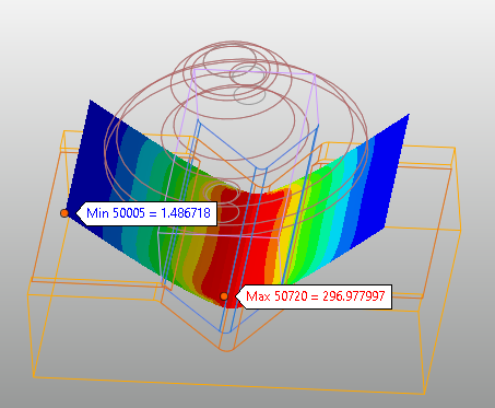
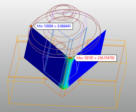
To see the contour result for Plate, as shown below, click the Wireframe tool in the Render Toolbar and run the animation.
You can see that, at 1.23 seconds, the Maximum Von-Mises Stress is approximately 296.98 MPa. After 1.53 seconds, approximately 236.35 MPa of residual stress remains.
7.2.6. Analyzing and Reviewing the Results
7.2.6.1. Task Objectives
This chapter analyzes the results of the two plastic analyses using different plastic materials and compares these analyses with the elastic analysis results.
7.2.6.2. Estimated Time to Complete
10 minutes
7.2.6.3. Analyzing the Plastic Analysis Results
7.2.6.3.1. Theoretical Explanation of Metal Plasticity
In the final analysis from the previous chapter, the metal plate modeled using a flexible body underwent plastic deformation due to the force of the punch striking it. The stress generated at the time of deformation is called yield stress. The stress can be expressed as a three-dimensional shape, such as a sphere or cube, by specifying the amount of stress along the X, Y, and Z axes in the three-dimensional space. The surface of such a sphere or cube is called the yield surface.
If the load is applied again to the flexible material constituting the metal plate after the material has passed from the elastic range into the plastic range, then the yield stress of the material increases along with the deformation of the material. This process is called hardening. Hardening is a fundamental property of a plastic material. RecurDyn can model two types of hardening.
The first is isotropic hardening, in which the yield surface of the stress sphere expands in all directions at the same rate. The second one is kinematic hardening, in which the size of the yield surface remains the same, but the center of the surface shifts.
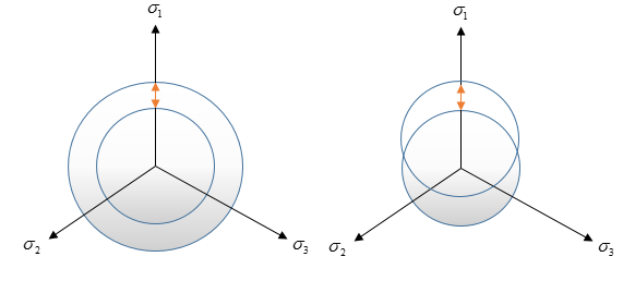
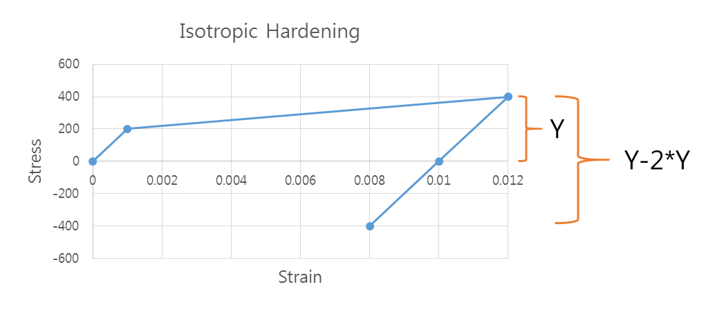
If only isotropic hardening is used, when the tensile load is removed and a compressive load is applied after the material has entered the plastic range, the yield stress of the material changes from +Y to –Y (Y - 2 × Y). During this process, the stress-strain relationship of the material shows linear elastic behavior.
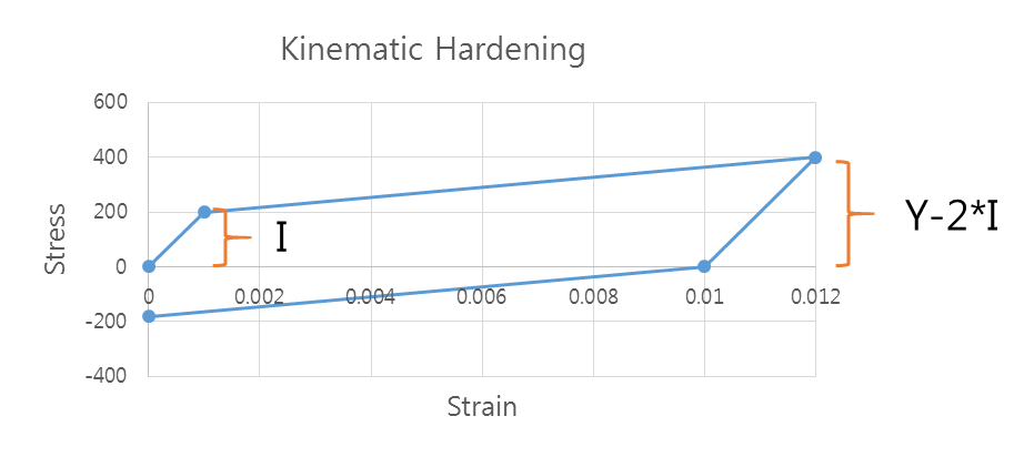
If only kinematic hardening is used, when the tensile load is removed and the compressive load is applied after the yield stress has exceeded the initial yield stress (I) and the material has entered the plastic range, the yield stress of the material changes from +Y to Y - 2 × I. During this process, the stress-strain relationship of the material shows linear elastic behavior.
RecurDyn provides two different hardening options. The first option allows for only using isotropic hardening. The second option is to use isotropic + kinematic hardening, which combines both isotropic hardening and kinematic hardening.
In the bending machine used for this tutorial, no additional force is applied after the punch falls on the metal plate to cause deformation. Therefore, there is not much physical difference between isotropic hardening and kinematic hardening. However, if you use a non-zero value for Kinematic Hardening (Hk), the effective hardening modulus changes, causing the slope in the plastic range (plastic modulus) to change and leading to different residual stress and permanent strain results.
7.2.6.3.2. Comparing the Results of Plastic Analyses (1) and (2)
7.2.6.3.3. To compare the plot results:
On the Analysis tab, in the Plot group, click the Plot Result function to enter Plot mode. The Modeling Window changes to the Plot Window.
On the Home tab, in the Import group, click the Import function.
In the Import dialog window, select the *.rplt files created from the two plastic analyses.
In the output folder created in the first analysis, select Isotropic_Plasticity.rplt.
Click the Import function again and, in the output folder created after the second simulation, select Isotropic_Kinematic_Plasticity.rplt. (If you entered Plot mode directly after finishing the Isotropic+Kinematic analysis, then this file is imported automatically.)
As shown in the figure below, the data from both rplt files appears in the Database Window.
Click the + button to the left of Isotropic_Plasticity. In the expanded tree, click the + button to the left of FFlex_Bodies -> Plate.Output1 -> Plate_Node5032 -> Shell -> Bottom, and then select EMISES_T.
Right-click EMISES_T to display the context menu, and then click Multi Draw.
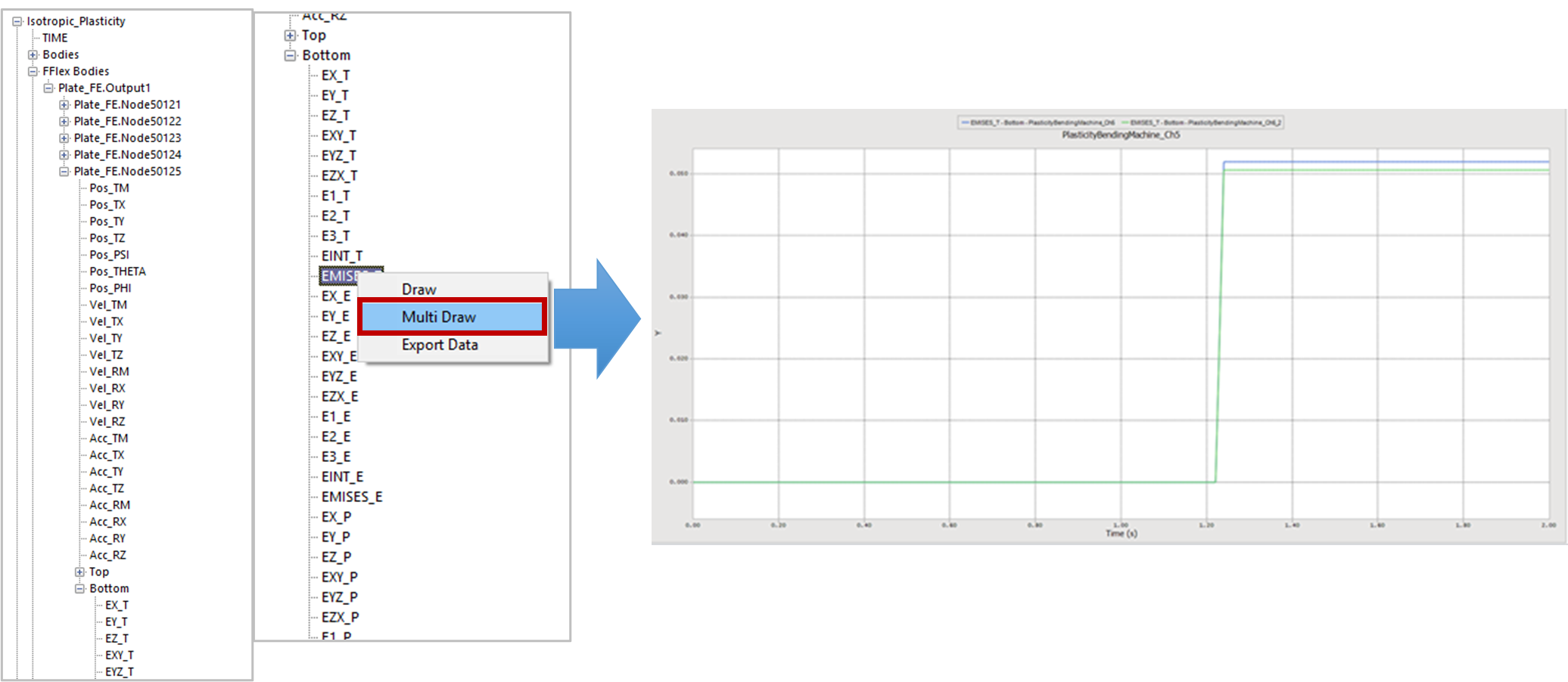
Two graphs appear in the Plot Window, as shown in the figures to the below.
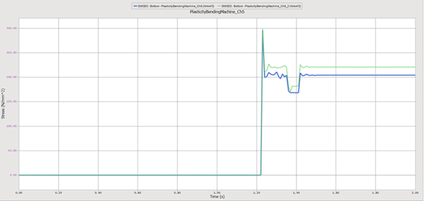
To match the figure shown on the below, right-click SMISES instead of EMISES_T in step 3 and select Multi Draw.
7.2.6.3.4. Analyzing the Results
The graphs drawn in the preceding procedure indicate the following:
The total strain is composed of the combination of plastic strain and elastic strain. The plastic strain causes the permanent deformation of the metal plate. Also, a difference can be detected between the behavior of plasticity with isotropic hardening and plasticity with isotropic + kinematic hardening. As was explained earlier, this is due to the difference in the slope of the plastic range.
As you can see in the Von-Mises stress results, the metal plate maintains a certain residual stress after deformation of the plate occurs due to outside impact.
7.2.6.4. For Reference
7.2.6.4.1. Multi-linear Models
The stress-strain relationship for the plastic range can be expressed using a formula. This tutorial used a multi-linear model that calculates the plastic modulus using multiple linear data. This method extracts the plastic strain and yield stress values from empirical results obtained from experiments and uses the values to generate a multi-linear model.
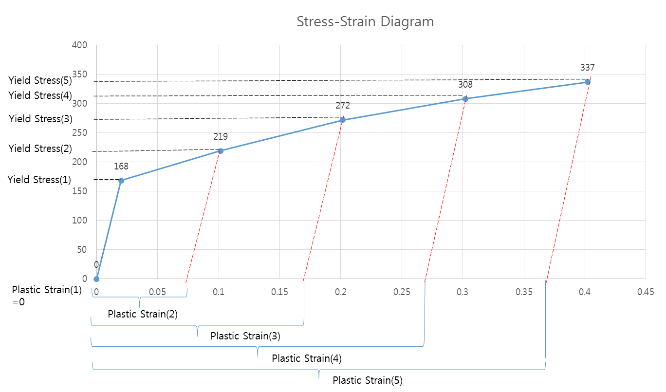
As shown in the figure above, you can obtain the Plastic Strain(x) and Yield Stress(y) values through experiments and enter the values in the Multi-linear group of the Plastic - Isotropic dialog window to create the blue stress-strain graph. In the stress-strain graph, the strain in the plastic range is the total strain that consists of both the plastic strain and elastic strain. Therefore, you must ensure that you enter only the plastic strain when you enter the data in the Multi-linear group. In the experiment, you can obtain the plastic strain by applying a load larger than the yield stress and measuring the degree of deformation in the material.