3.4. Suspension System Tutorial (AutoDesign)

3.4.1. Outline of Tutorial Sample D

Model

Description

Sample D

Suspension System Design Problem: This design has two design objectives. Also, it has 27 design variables. The design goal is to minimize the Yaw-range and the Roll-Range of tire motion. This problem is not easy because it is a multi-objective problem and has too many design variables. In general, other design tools employ D-Optimal design or Latin Hypercube for constructing the meta model. Suppose that construct a quadratic response surface model, D-optimal design fundamentally requires 406 sampling points, which is evaluate by using 1+2*27+27*26/2. AutoDesign uses however only 44 evaluations to solve the problem without variable screening. Key Point: Study the concept of multi-objective optimization and the procedure of screening design variables.

3.4.2. Suspension System Design Problem

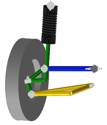
Let’s consider the simple model of car suspension system. The system has 5 components such as arm, tie rod, knuckle, shock absorber damper and tire. When the tire moves along vertical direction, the simulation shows the damping process and kinematical motion.

All the design variables are the geometric coordinates of joints. The design objective is to minimize the first rotational Yaw-Roll of tire.

This problem has 27 design variables for 9 joints. Nevertheless, we will try to minimize the Yaw-range and the Roll- range directly. In other words, design variable screening is not used. Next, we will re-try to solve the same problem after screening the design variables. Then, the optimization results will be compared.

Open files related in Sample-E
Sample		<InstallDir>\Help\Tutorial\AutoDesign\SuspensionSystem\Examples\SAMPLE_D0.rdyn
Solution	1	<InstallDir>\Help\Tutorial\AutoDesign\SuspensionSystem\Solutions\SAMPLE_D0.rdyn
	2	<InstallDir>\Help\Tutorial\AutoDesign\SuspensionSystem\Solutions\SAMPLE_D1.rdyn
	3	<InstallDir>\Help\Tutorial\AutoDesign\SuspensionSystem\Solutions\SAMPLE_D2.rdyn

Note

If you change the file path at discretion, it can be located in any folder that you specify.

3.4.3. Loading the Model and Viewing the Yaw & Roll ranges

3.4.3.1. To load the base model and view the animation:

1. On your Desktop, double-click the RecurDyn tool. RecurDyn starts and the Start RecurDyn dialog box appears.

2. Close Start RecurDyn dialog box. You will use an existing model.

3. In the toolbar, click the Open tool and select Sample_D0.rdyn from the same directory where this tutorial is located. The suspension system appears in the modeling window.

4. Click Dynamic/Kinematic.

5. Click Simulate.

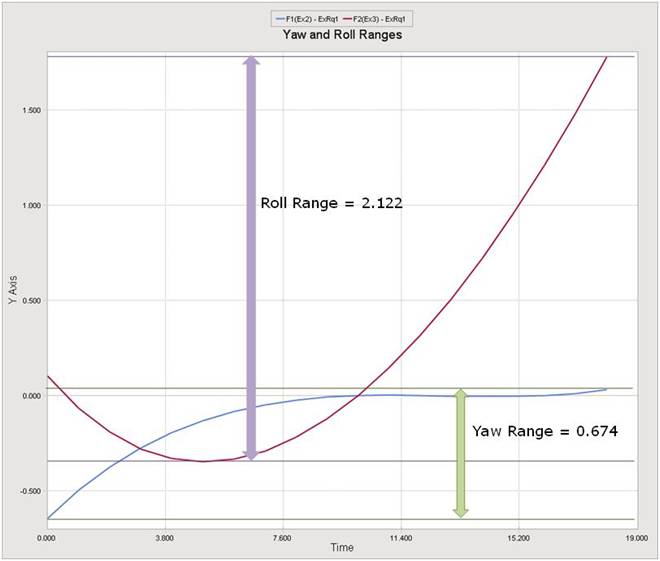
6. Click the Plot Result function on the ribbon menu. Then, window is switched. In right side, you can see plot database. If it is not shown, check the database window in View menu. Expression 2 & 3 are Yaw and Roll angles.

   

3.4.4. Defining the design variables

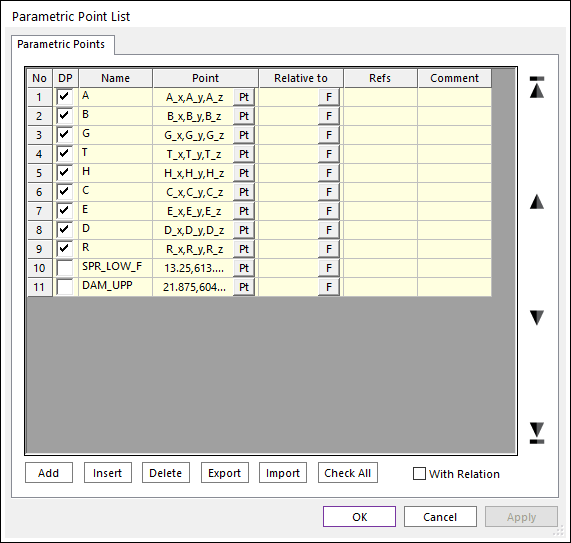
All geometric coordinates of joints are defined by using Parametric Points shown at the below figure. In Figure, they are represented as A_x, A_y, …, R_y and R_z.

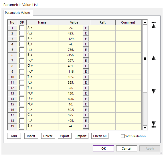
Next, the parametric values are defined in the Parametric Value menu in Subentity.

All the above relations have defined in the model SAMPLE_D.rdyn.

Next, select the Design Parameter menu.

Then, you can see that 27 parametric values are linked by design parameters as shown below.

3.4.5. Defining the performance index

Let’s consider the performance indexes. We will minimize the Yaw and Roll ranges during tire moves vertical direction. As RD does not provide those values directly, we should evaluate them by using Expression and Variable Equation.

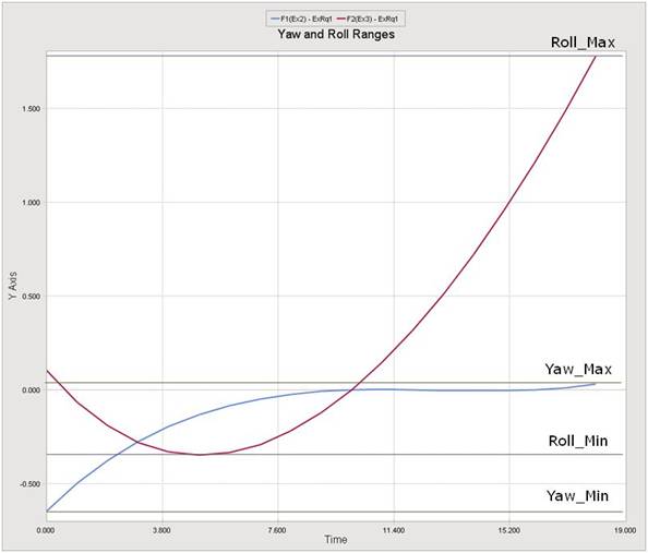
In order to evaluate them, we evaluate the minimum and the maximum values for Yaw and Roll angles. Then, the deviations between Max and Min are the ranges for them.

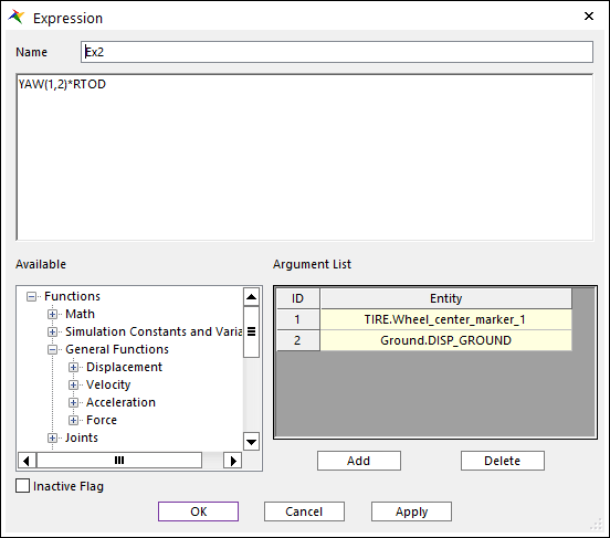
• Step 1: Create the Expression for Yaw and Roll angles. The following figures show the expressions to save Yaw and Roll angles.

  

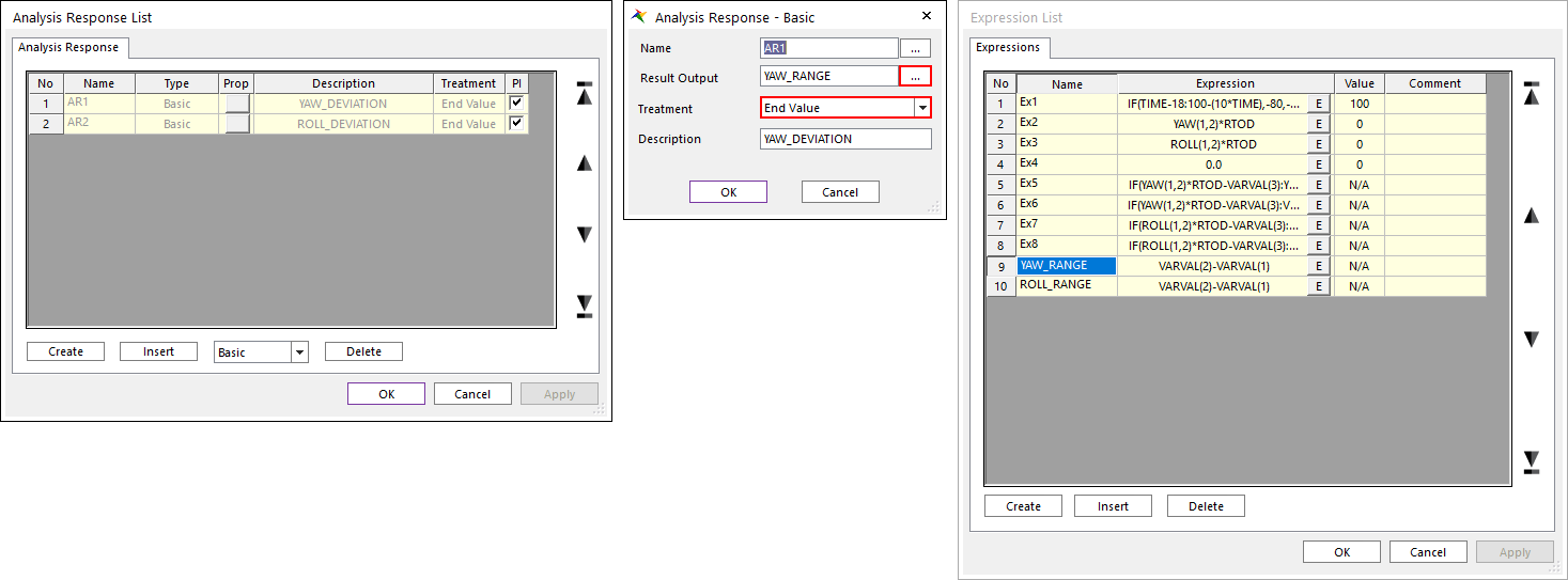
• Step 2: By using Expression, YAW_DEVIATION and ROLL_DEVIATION are defined. Then, you can define them as analysis responses at Analysis Response in AutoDesign. The following figure shows this process.

  

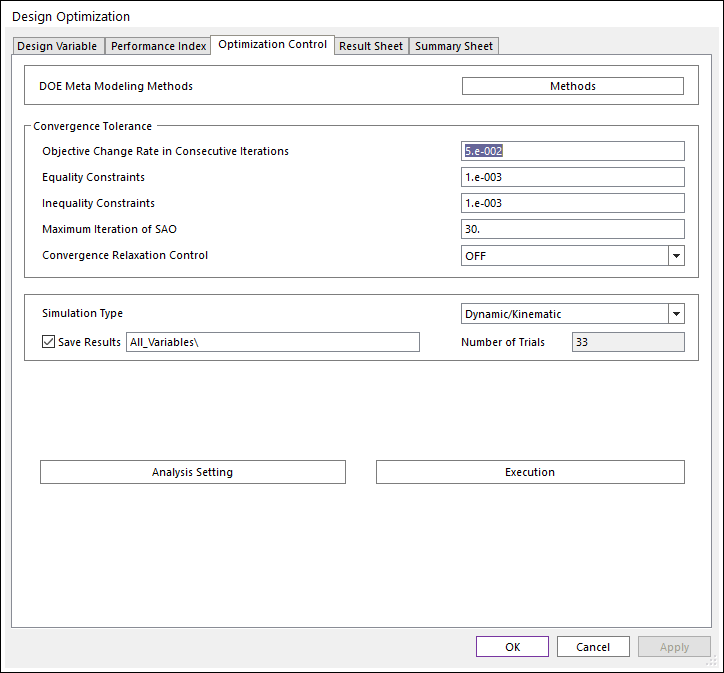
3.4.6. Running a Design Optimization

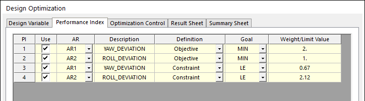
When you select the Design Optimization, all the design variables, check in DV, will be included in the design. The performance index however will be empty. Then, you add ARs to the Performance Index.

The optimization problem is to minimize the Yaw Range and the Roll Range while satisfying those two ranges less than them of the current design. Also, we think that Yaw Range is more important than Roll Range. Thus, its’ weight is twice greater than that of Roll.

Minimize Yaw_Deviation*2 & Roll_Deviation

subject to

Yaw_Deviation =< 0.67

Roll_Deviation =< 2.12,

where the values of 0.67 and 2.12 are the range values for the current design. Those two inequality constraints seem to be redundant because two objectives should be minimized. It is however not guaranteed. Thus, it is difficult to solve multi-objective optimization problem. In the Part II manual: Guideline for AutoDesign, the chapter 5 explains the multi-objective optimization.

Let’s consider the above design problem from the view of multi-objective optimization process. If necessary, let’s denote \({{f}_{1}}\) =Yaw_Deviation and \({{f}_{2}}\) =Roll_Deviation. When the initial samples construct the approximate functions of \({{f}_{2}}\) =Roll_Deviation and \({{f}_{2}}\) =Roll_Deviation, which are called as metamodels. Then, \(f_{1}^{*}\) and \(f_{2}^{*}\) is the minimum values from the initial samples.

\(Min\max \left\{ \left( \frac{{{f}_{1}}(\mathbf{x})-f_{1}^{*}}{f_{1}^{*}} \right),\left( \frac{{{f}_{2}}(\mathbf{x})-f_{2}^{*}}{f_{2}^{*}} \right) \right\}\)

Thus, the quality of multi-objectives optimization depends on the number of initial samples. Unfortunately, this problem has 27 design variables, which requires too many sample points. Those two inequality constraints can avoid the pre-mature convergence, even though the number of initial samples is minimized.

3.4.6.1. Let’s start to solve the multi-objective optimization problem:

1. Click the Performance Index page. Then, define the above optimization formulation as follows:

   

2. Click the Optimization Control page. The default values are directly used. Then, click Execution.

   

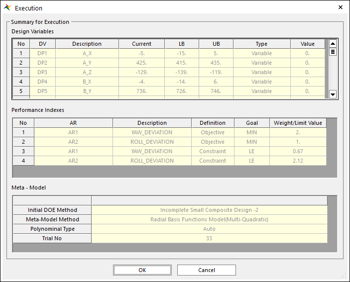
   Then, you can see the summary of design formulation. Check Design Variables, Performance Index and Meta-Model information. If all information is correct, then click OK. Then, optimization process is progressed.

   

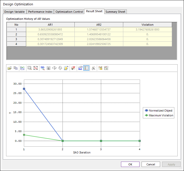
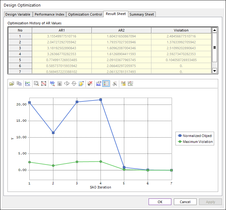
3. When the optimization process is completed, the Result Sheet page is automatically shown. The optimization process is converged in 4 iterations. Thus, AutoDesign solves the suspension system design having 27 design variables only for 37 analyses that includes 33 analyses for the initial sampling points. The final design gives that AR1=0.651 and AR2=1.407, which can minimize the Yaw deviation by 0.3 % and the Roll deviation by 33.7 %.

   • Convergence History

     

   • Summary Sheet

     

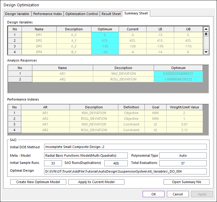
   In the summary sheet, shown in the above, is newly provided. The optimization results are summarized in the design variables and analysis responses lists. Also, the SAO information is summarized, which shows that SAO requires 4 iterations. Thus, the number of total evaluations is 37. And the analysis result of optimal design is DO_004.

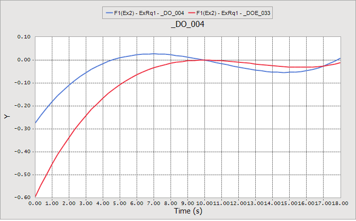
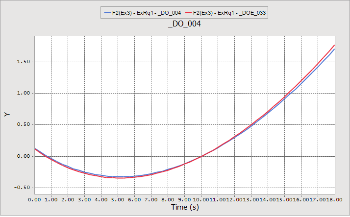
4. Finally, let’s compare the yaw and roll ranges for the initial design and the final design. DO_004 is the final design. Also, DOE33 is the initial design. The following figures show those comparisons. When the ISCD-1 and ISCD-2 compose the initial samples, the final one of the initial samples is the current design. In the following figures, the red color line is an optimum result.

   • Yaw(Toe)

     

   • Roll(Camber)

     

3.4.7. Design Optimization with Screening Variables

Now, let’s compare the optimization results for considering all design variables and the screened design variables. Thus, save the model file Sample_D0.rdyn as Sample_D1.rdyn and delete all the results in the Simulation History.

First, let’s try to screen the design variables. As screening is based on the effect analysis results, you select the design study in AutoDesign. Following steps explain the screening process:

1. Enter the Design Study menu.

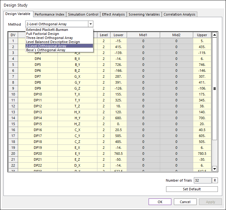
2. Then, you can see the list of design variables in the Design Variable page. As the number of design variables is 27, we select the 2-Level Orthogonal Array to reduce the number of trials. If 3-Level Orthogonal Array is selected, the number of trials is 81.

   

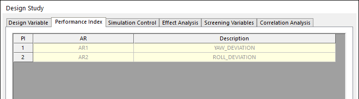
3. Next, in the Performance Index page, two analysis responses such as AR1 and AR2 will be shown. If they are not, you retry to make Sample_D1.rdyn from Sample_D0.rdyn.

   

4. Next, click the Simulation Control page. If you save the analysis results each trial, check the Save Results and enter the Folder name. Then, click Execution.

   

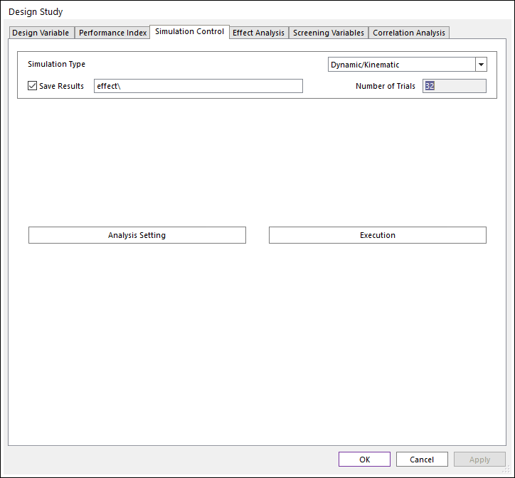
5. After all analyses have been completed, the design study window is activated. Then, click the Effect Analysis page. Then, you can see the effect analysis chart by checking the check boxes in the Effect Values column and clicking Draw. The effect analysis results are shown as follows:

   

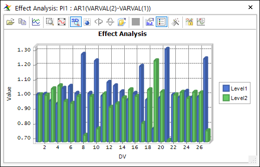
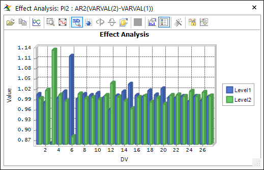
   Two figures show that the different variables are sensitive to PI_1 and PI_2. Generally, users select the sensitive variables from the above charts. It is however not easy. Thus, AutoDesign provides a statistical guideline for screening variables.

6. Click the Screening Variables page. Then, select AR_1 in the PI box. Then, you can see the scatter points. The right positioned points are more sensitive to the left ones. Move the controller to divide design variable groups. Then, the Cutoff Value as 0.3 and click Screening DV.

   

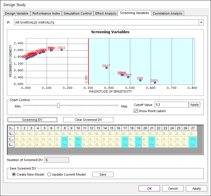
   Then, the red line divides the scatter points into two groups. The right group is the remaining variables. Then, the screened variables are marked as On. Others are done as Off.

   Next, select AR2 in the PI box and do the same process similarly except defining Cutoff Value as 0.06. Then, the screened variables are summarized as follows:

   

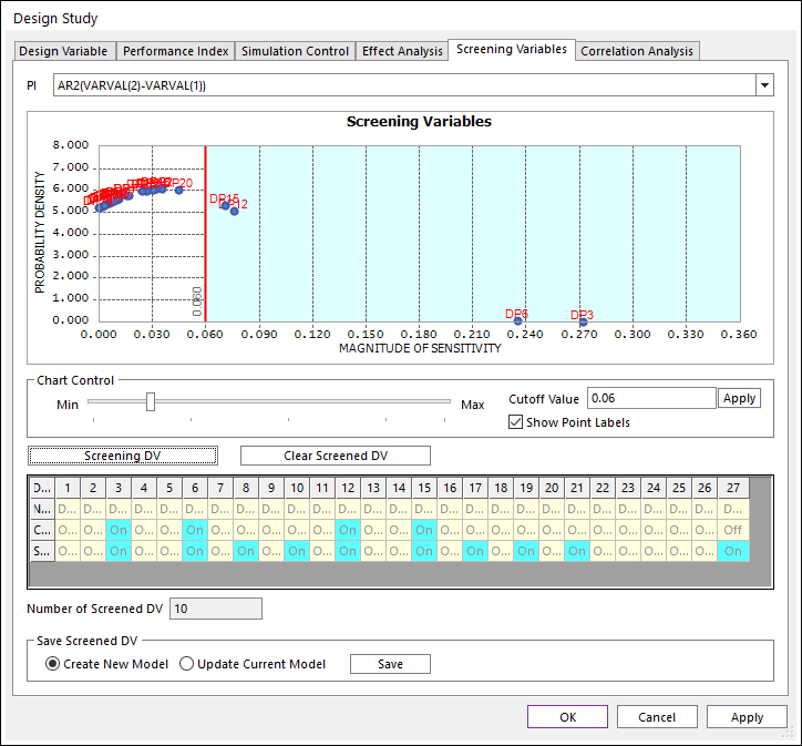
   The screening DV gives that the active design variables (DV) are DP3, DP6, DP8, DP10, DP12, DP15, DP17, DP19, DP21, and DP27.

   Now, create the new model by clicking Save with checking Create New Model. The new model file name is Sample_D2.rdyn.

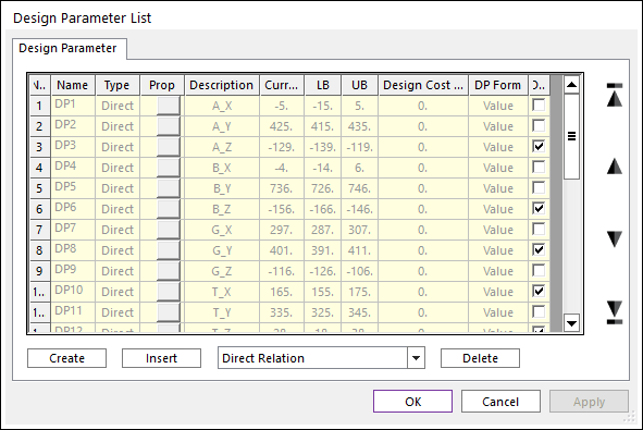
7. Now, you can see that the model file is changed as Sample_D2.rdyn. Click the Design Parameter function in AutoDesign. Unlike the model Sample_D1.rdyn, the screened variables are only checked in DV column. This represents that DV1=DP3, DV2=DP6, DV3=DP8, DV4=DP10, DV5=DP12, DV6=DP15, DV7=DP17, DV8=DP19, DV9=DP21, and DV10=DP27. Most of the active design parameters are z-coordinate values.

   

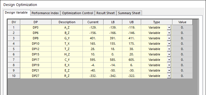
8. Next, Click the Design Optimization function. Then, the screened variables are shown as follows:

   

9. Click the Performance Index page. The optimization formulation will be the same as that of Sample_D1.rdyn. Let’s use the same formulation.

   

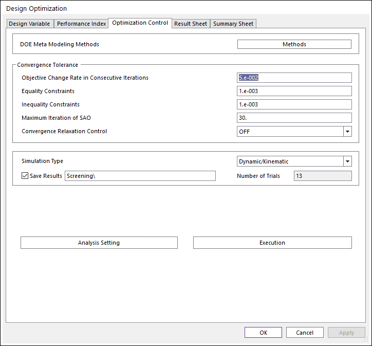
10. In the Optimization Control page, all the convergence tolerances use the default values. The result files are saved in the folder Screening.

    

11. After the optimization is completed, let’s see the result sheet. AutoDesign is converged in 5 iterations. The optimized AR1 and AR2 are 0.586 and 1.503, respectively. AR1 and AR2 are similar to those of the design without screening.

    • Convergence History

      

    Unlike the convergence history for the design problem without screening, the above convergence history simply decreased. Let’s compare the summary of two optimization problems.

    	With Screening	Without Screening
    Number of design variables	10	27
    Initial samples	13	33
    Number of SAO runs	5(1)	4
    Samples for screening	32
    Optimum response	0.586, 1.503	0.651, 1.407