1.5. Dipper Stick with Bucket Tutorial (Professional)
1.5.1. Getting Started
1.5.1.1. Objective
This tutorial familiarizes you with the methods used to design dynamic systems. This includes parametric modeling using parametric points and values at both the main and subsystem levels, parametric bodies, and expressions. It also includes setting up design variables, performance indexes, and a design study. This tutorial concludes with instructions for simulating the best candidate designs in batch mode and plotting their results simultaneously.
1.5.1.2. Model Used
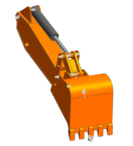
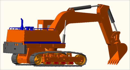
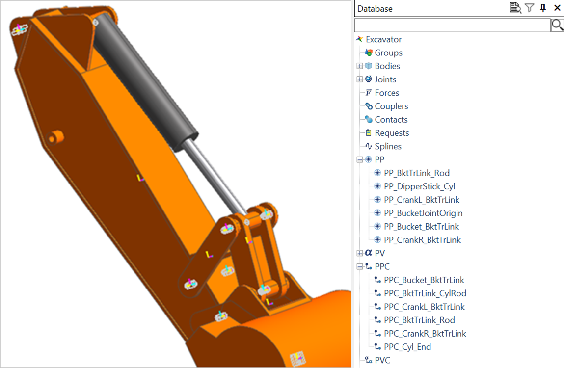
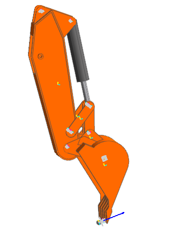
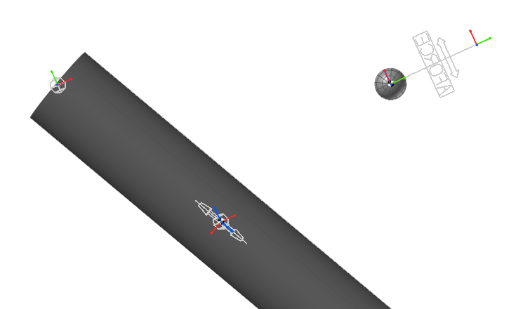
The model used in this tutorial comes from an excavator. You will look specifically at the design of the four-bar linkage connecting the hydraulic cylinder and the bucket to the dipper stick as shown in the following figure.
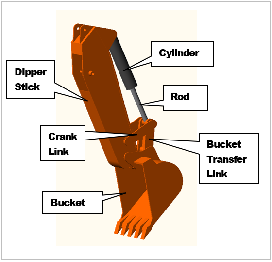
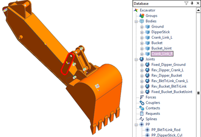
For ease of working with the model and to decrease the simulation time, we only include the dipper stick and the bodies of the bucket linkage in this tutorial. The next figure shows the simplified model and the names of the major bodies and links.
The objective of the design study is to decrease the amount of power required to drive the bucket through a dig and return motion, while at the same time maintaining a high range of motion for the bucket. The design variables are the length of the crank link and the position of the bucket joint where it connects to the bucket transfer link. While varying these two design variables the initial length of the hydraulic cylinder should be unaltered so that the same hydraulic cylinder can be used in the modified design. This makes the comparison between designs more objective because the same actuator is used consistently.
The equations to enforce this constraint are beyond the scope of this tutorial, so they are provided for you in the base model. In fact, almost all of the parametric points and values are provided in the base model, and only a few were left out so that this tutorial could be completed in a reasonable amount of time while still showing the methods used in creating this model. If you are interested, you should take some time after completing this tutorial to go back through the model and see what was provided for you. This will be easier to understand after having seen the steps used to create the additional components of the model as presented in this tutorial.
1.5.1.3. Audience
This tutorial is intended for experienced users of RecurDyn. All new tasks are explained carefully.
1.5.1.4. Prerequisites
Users should first work through the 3D Crank-Slider, Engine with Propeller, and Pinball (2D contact) tutorials, or the equivalent. We assume that you have a basic knowledge of physics.
Procedures
The tutorial is comprised of the following procedures. The estimated time to complete each procedure is shown in the table below.
If you do not want to go through the model construction portions of the tutorial, we have provided a completed model so that you can begin working in Chapter 6, Creating an Expression. Simply load Excavator_final.rdyn from the tutorial directory and start with the instructions in Chapter 6.
Procedures |
Time (minutes) |
Creating the link |
15 |
Creating the hydraulic cylinder |
15 |
Adding motion to the hydraulic cylinder |
15 |
Adding a load to the tip of the bucket |
15 |
Calculating power consumption |
15 |
Calculating the bucket’s range of motion |
15 |
Running and analyzing a design study |
15 |
Running a simulation in batch mode |
15 |
Total |
120 |
1.5.1.5. Estimated Time to Complete
This tutorial takes approximately two hours to complete if you perform all the tasks, and one hour if you begin at Chapter 6 when the model construction is complete.
1.5.2. Creating the Link
1.5.2.1. Task Objective
Learn how to create a parametric point and create and modify the right-side link. You will also attach this link to the subsystem using revolute joints.
1.5.2.2. Estimated Time to Complete
15 minutes
1.5.2.3. Starting RecurDyn
1.5.2.3.1. To start RecurDyn and open the base model:
On your Desktop, double-click the RecurDyn icon. RecurDyn starts and the Start RecurDyn dialog box appears.
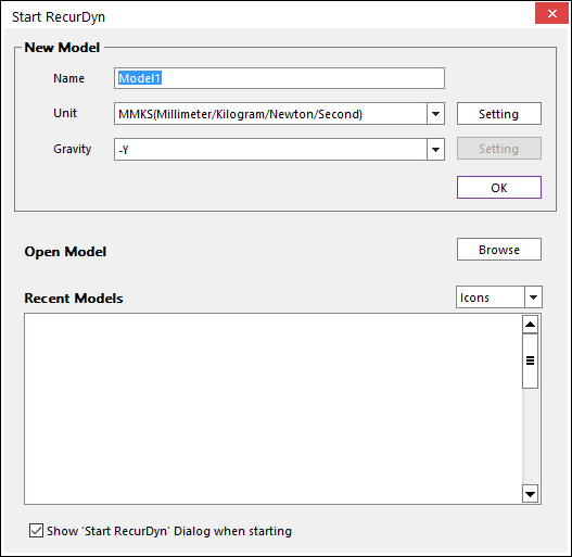
Close Start RecurDyn dialog box. You will use an existing model.
- In the Quick Access Toolbar, click the Open and select Excavator.rdyn.(The file path: <InstallDir>\Help\Tutorial\Professional\DipperStickWithBucket)The excavator appears in the modeling window. Note that the hydraulic cylinder is missing. You will import it in the next chapter.
1.5.2.4. Setting the Working Plane
After opening the model, you will notice that the working plane is the XZ plane, as indicated by the grid. This is a good working plane orientation because all the motions you are concerned with occur in this plane.
To ensure that all the components you create in this tutorial will be in the correct orientation, always make sure that the model’s working plane is set to the XZ plane. If it is not, you can reset it to the correct orientation by clicking the Working Plane tool and selecting the XZ plane.
1.5.2.5. Creating a Parametric Point
1.5.2.5.1. To create a parametric point:
From the Parameter group in the SubEntity tab, click the Parametric Point function.
Click Add to create a new parametric point.
Change the name of the point to PP_CrankR_BktTrLink.
Double-click the cell shown in grey in the picture on the below, and enter the following in cell to define the location of the point:
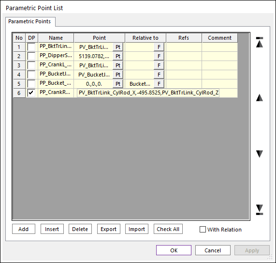
PV_BktTrLink_CylRod_X,-495.8525,PV_BktTrLink_CylRod_Z
This means that the x-location of this parametric point is determined by the parametric value PV_BktTrLink_CylRod_X and the z-location is determined by PV_BktTrLink_CylRod_Z. The y-location is set to be the center of the link you are going to create.
Click OK.
Parametric points allow you to parametrically change the configuration or design of the model in an automated way. The equations used to calculate the parametric values for the x and z locations of the point you created are functions of two other parametric values, the crank length and the bucket joint angle. For the crank length you are creating here, if you want the end point of the link to move when you change the crank length, you need to define the end point using a parametric point.
1.5.2.5.2. To link the BkTrLink subsystem:
From the Parameter group in the SubEntity tab, click the Parametric Point Connector function.
Click Add to create a new PPC.
Double-click PPC1 and rename the PPC to PPC_CrankR_BktTrLink.
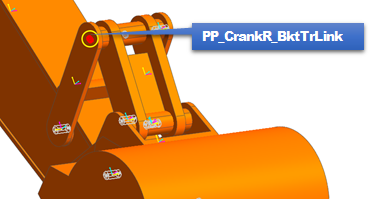
In the Point text box, select PP_CrankR_BktTrLink, by doing one of the following:
Double-click the text box and enter the name of the parametric point.
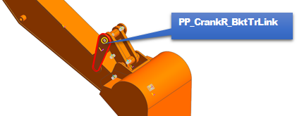
Click Pt and then click the parametric point in the Working window as shown in the figure as above.
Click Pt and then click & drag the parametric point named PP_CrankR_BktTrLink in the Database window to Input Window Toolbar.
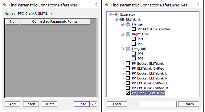
Click the More button (…) in the Refs column.
Click the Continue button (>>) in the bottom right corner.
In the dialog box that appears, scroll down and click the box next to PP_CrankR_BktTrLink under BktTrLink.
Click Load to enter the appropriate data in the dialog box on the left and click the Close button to exit the dialog boxes. See the figure below.
1.5.2.6. Creating the Right-Side Crank Link
1.5.2.6.1. To create the right-side crank link:
From the Marker and Body group in the Professional tab, click the Link function.
Set the Creation Method toolbar to Point, Point, HalfDepth.
Enter the following coordinates into the Input Window toolbar for the first link point:
5506.1017, -495.8525, 2231.9958
Click the newly created parametric point (PP_CrankR_BktTrLink) to select the second link point.
Set the thickness of the link by entering 17.5 for the HalfDepth in the Modeling Input toolbar. The link should look like the following figure.
Right-click the link and click Properties.
On the General page, change the name from Body1 to Crank_Link_R.
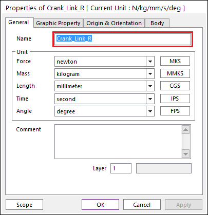
Click OK.
1.5.2.7. Modifying the Link Shape and Color
Now, you will modify the link shape and color to make it match the rest of the model.
1.5.2.7.1. To modify the link shape and color:
Double-click the link to enter Body Edit Mode.
Right-click the link and click Properties.
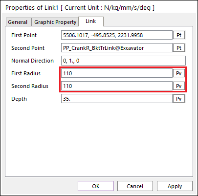
First, modify the end radii to match the other crank link. Click the Link page to modify the dimensions.
Enter 110 for First Radius and Second Radius.
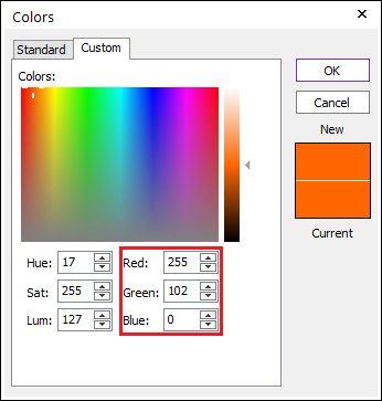
Click the Graphic Property page to modify the color.
Set Color to More Colors.
In the dialog box that appears for changing the color, click the Custom page and enter the following:
Red: 255
Green: 102
Blue: 0
Tip
You do not need to modify the Hue, Saturation (Sat), or Luminosity (Lum) because they update automatically when you change the RGB values.
Click OK.
Click OK again until back in Body Edit Mode and all the dialog boxes are closed.
Click the Exit function to exit Body Edit Mode.
Your model should look like the figure on the below.
1.5.2.8. Attaching the Link
You now attach the link to the rest of the subsystem using revolute joints.
1.5.2.8.1. To attach the link:
From the Joint group in the Professional tab, click the Revolute Joint function.
Set the Creation Method to Body, Body, Point.
Create a joint at the bottom of the link by selecting the link (Crank_Link_R), then the DipperStick and entering the following point information:
5506.1017, -477.85255, 2231.9959
Tip
As long as the working grid is in the XZ plane (which it should be by default), the orientation of the joint will be correct.
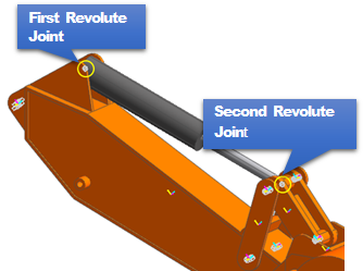
Now you will create the second joint at the top of the link in the same way, but because the bucket transfer link (BktTrLink) is part of a subsystem, you must hold down the Shift key while selecting BktTrLink as the second body for the joint.
From the Joint group in the Professional tab, click the Revolute Joint function.
Choose Crank_Link_R as the first body, the shaft at the top of the BktTrLink_CylRod_Cylinder@BktTrLink subsystem as the second (while holding down the Shift key), and then click on the newly created point PP_CrankR_BktTrLink as the location for the joint.
You must choose the parametric point as the location of the joint so the location of the joint will update when the parametric point is moved.
Save your model very under Desktop directory named Excavator. (C:\Users\PC-Name\Desktop\Excavator)
1.5.3. Creating the Hydraulic Cylinder
1.5.3.1. Task Objective
In this chapter, you will import the hydraulic cylinder and link it to the model using parametric points and test the model.
1.5.3.2. Estimated Time to Complete
15 minutes
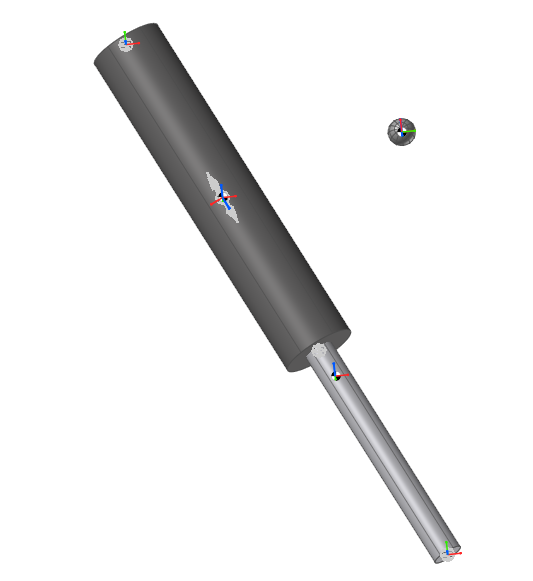
1.5.3.3. Importing the Generic Hydraulic Cylinder Subsystem
1.5.3.3.1. To import the hydraulic cylinder subsystem:
From the File menu, click the Import function.

- From the list of files, choose Hydraulic_Cylinder.rdsb.(The file path: <InstallDir>\Help\Tutorial\Professional\DipperStickWithBucket)
Click Open.
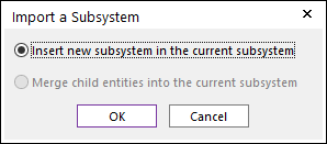
In the dialog box that appears, click OK to create a new subsystem.
Now, you will rename the imported subsystem:
In the Database window, right-click SubSystem1 and select Properties.
Click the General page and enter HydraulicCylinder as its name as shown in the figure on the below.
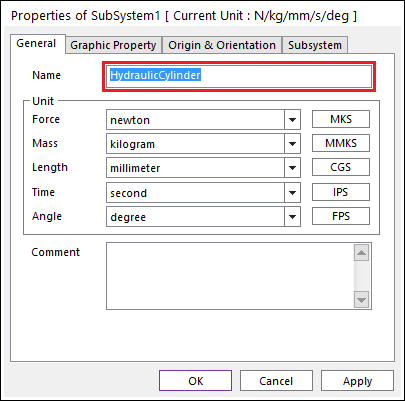
Click OK.
The hydraulic cylinder you just imported already has a number of parametric points, parametric values, and expressions in it. They were created to make this hydraulic cylinder totally parametric so it can be used in any model. All you need to do is to create parametric points at the model level for the end points of the hydraulic cylinder and then connect them to the subsystem using parametric point connectors, which you will do next.
1.5.3.4. Setting the Location of the Hydraulic Cylinder Subsystem
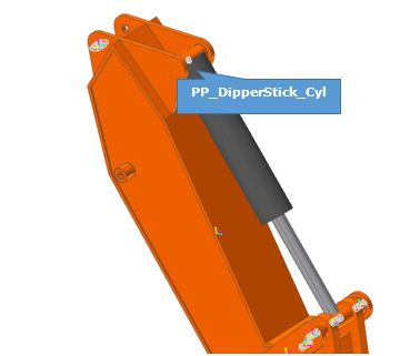
In this section, you set the location of the hydraulic cylinder subsystem by linking the parametric points at the main model level to parametric points in the hydraulic cylinder subsystem, using parametric point connectors (PPC). The parametric points at the main model level are the first two on the list of parametric points, PP_BktTrLink_Rod and PP_DipperStick_Cyl, and their names indicate what they were made to connect.
1.5.3.4.1. To link the hydraulic cylinder subsystem:
From the Parameter group in the SubEntity tab, click the Parametric Point Connector function.
Click Add to create a new PPC.
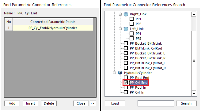
Double-click PPC1 and rename the PPC to PPC_Cyl_End.
In the Point text box, select PP_DipperStick_Cyl, by doing one of the following:
Double-click the text box and enter the name of the parametric point.
Click Pt and then click the parametric point in the Working window as shown in the figure as above.
Click Pt and then click & drag the parametric point named PP_DipperStick_Cyl in the Database window to Input Window Toolbar.
Click the More button (…) in the Refs column.
Click the Continue button (>>) in the bottom right corner.
In the dialog box that appears, scroll down and click the box next to PP_Cyl_End under HydraulicCylinder.
Click Load to enter the appropriate data in the dialog box on the left and click the Close button to exit the dialog boxes. See the figure below.
Perform the same set of operations for the other end of the hydraulic cylinder, but this time select the PPC to PPC_BktTrLink_Rod. This PPC should reference PP_Rod_End from the HydraulicCylinder subsystem.
When you click OK to accept your changes in the Parametric Point Connector List dialog box, the hydraulic cylinder automatically moves itself into the correct position as shown in the following figure.
1.5.3.5. Attaching the Hydraulic Cylinder to the Model
You will now attach the hydraulic cylinder subsystem to the model with two revolute joints:
The first revolute joint connects the dipper and the cylinder
The second revolute joint connects the top shaft of the bucket transfer link and the rod.
1.5.3.5.1. To attach the hydraulic cylinder:
From the Joint group in the Professional tab, click the Revolute Joint function.
Set the Creation Method to Body, Body, Point.
Click DipperStick and while holding down the Shift key, click the Cylinder from the HydraulicCylinder subsystem. Then, click the parametric point at the end of the cylinder (PP_Dipperstick_Cyl) as that location of the joint.
Follow the same procedure to create the revolute joint at the other end of the hydraulic cylinder. This time, while holding down the Shift key, click Rod from the HydraulicCylinder subsystem and then the BktTrLink_CylRod_Cylinder from the BktTrLink subsystem. Finally, release the Shift key and click the parametric point located at the end of the rod (PP_BktTrLink_Rod).
Make sure to release the Shift key before selecting the joint location because the parametric point you want is located at the system level.
1.5.3.6. Exercising the Model
Having completed the previous steps, your model should now update the geometry automatically when the values for PV_DeltaCrankLength and PV_BucketJointAngleDeg are changed. Try this to ensure that it is working (you can choose not to do this step without losing continuity).
1.5.3.6.1. To exercise the model:
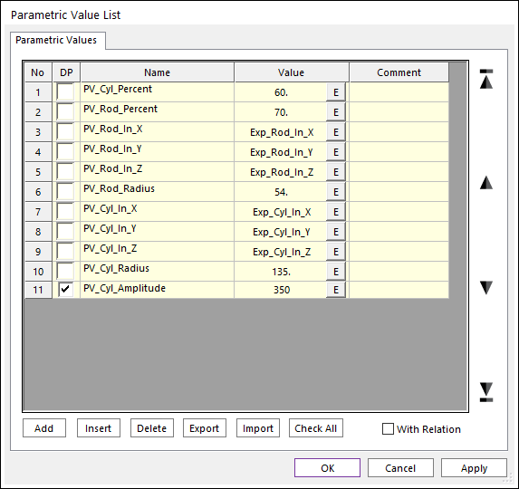
In the Database window, double-click any of the parametric values (PVs) to display the Parametric Value List dialog box shown in the figure on the below.
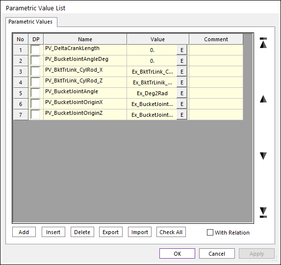
Try changing the value for PV_DeltaCrankLength to a value between -150 and 150 and then click Apply to see the model update.
Similarly, try changing the value for PV_BucketJointAngleDeg from 0. to a value between -15 and 15 and then click Apply to see the model update.
Tip
Why is the fixed joint between the bucket joint and the bucket located out in space, rather than within the intersection of these two bodies?While exercising the model, you might notice that this joint location is not where you would expect the joint forces to actually occur. This location was chosen to facilitate being able to specify the bucket joint position easily with only an angle. This location is also acceptable because in this model, you are not concerned with the reaction forces at this joint, and the location of a fixed joint does not influence the behavior of the two joined rigid bodies with respect to each other.Tip
Other values could be chosen for these PVs but the model will not necessarily update appropriately because the expressions and parametric entities were not created to go beyond these limits.
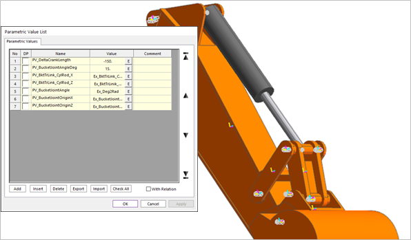
For comparison, the figure below shows what the model should look like when the values are set to -150 and 15, respectively.
When you are finished experimenting, be sure to change the values back to zero for both PVs and click OK.
Save your model.
1.5.4. Add Motion to the Hydraulic Cylinder
1.5.4.1. Task Objective
In this chapter, you will add translational motion to the hydraulic cylinder to drive the bucket rotation. You will do this at the HydraulicCylinder subsystem level where the translational joint is located. You will define a parametric value in the subsystem and connect its value, using a parametric value connector, with a parametric amplitude that is defined at the system level.
1.5.4.2. Estimated Time to Complete
15 minutes
1.5.4.3. Creating a Parametric Value
You will first create a parametric value (PV) in the Hydraulic cylinder subsystem.
1.5.4.3.1. To create a PV:
Enter the Subsystem Edit Mode for the hydraulic cylinder. Either:
In the Working window, double-click the hydraulic cylinder.
In the Database window, right-click HydraulicCylinder and click Edit.
Only the hydraulic cylinder appears.
Open the Parametric Value List as described previously. (SubEntity > Parametric Value)
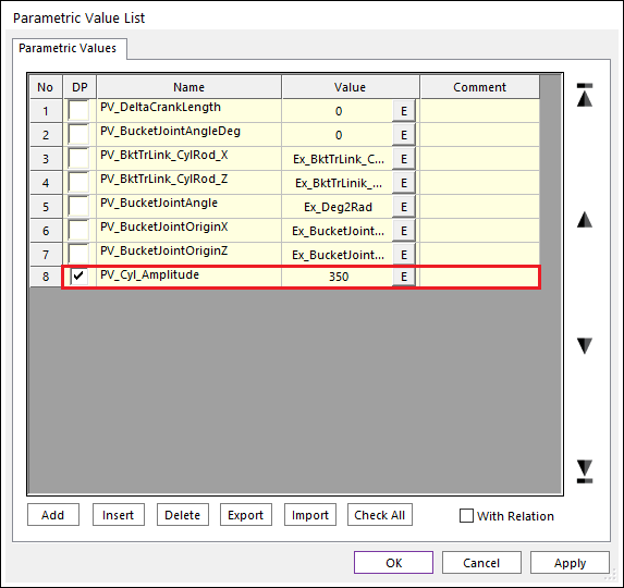
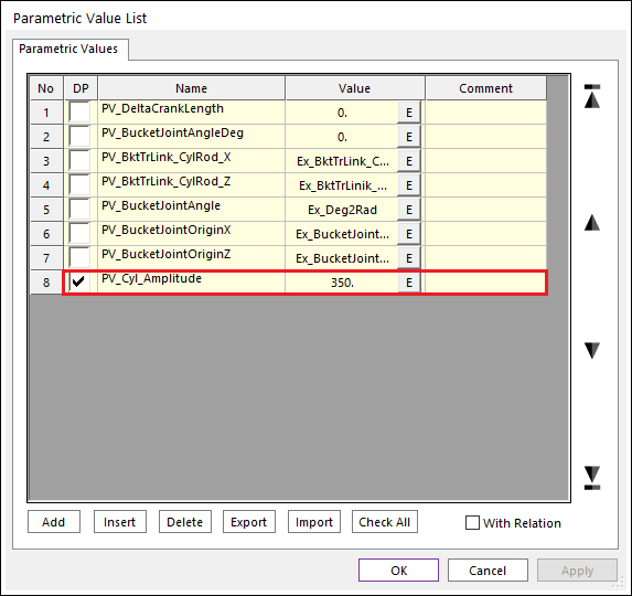
Click Add to create a new PV and rename it PV_Cyl_Amplitude as shown in the figure on the below.
Set the value to 350 (this means that the hydraulic cylinder will oscillate 350 mm in each direction during the simulation).
Click OK.
1.5.4.4. Adding Motion to the Translation Joint
You could define the needed motion in many different ways, ranging from something as simple as a sinusoidal displacement to something as complex as a cycloidal or modified trapezoidal displacement profile that limits the magnitude of the derivative of the acceleration (jerk) of the cylinder. Rather than use one of these motion definitions, you will use step changes in the joint velocity. This minimizes the jerk while still being a very simple profile (the Step function implemented in RecurDyn uses cubic functions at the corners of the step profile to minimize jerk).
1.5.4.4.1. To add motion:
In the Database Window, right-click TraJoint1 and select Properties.
Click Include Motion and then click Motion as shown in the figure on the below.
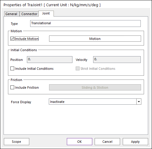
In the Motion dialog box that appears, set the motion to Velocity (the second drop-down box) and leave the initial position at 0.0 (the default).
Click EL to view the expression list from which you will define the velocity profile. A number of expressions already exist, but you will create a new one
Click Create.
Rename the expression Ex_StepCylVel and enter the following equation:
PV_Cyl_Amplitude*(STEP(TIME,0,0,0.1,-1) + STEP(TIME,1,0,1.1,2) +STEP(TIME,3,0,3.1,-2))
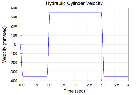
This equation will drive the joint at a speed of negative PV_Cyl_Amplitude per second for one second, then switch to driving at the same speed in the positive direction for two seconds, and then switch back to negative for one more second, returning it to its original position. The plot on the below shows the resulting function when PV_Cyl_Amplitude has a value of 350.
Click OK to accept the expression definition and then click OK three more times to accept all of the steps in creating the joint motion.
Click the Exit arrow to exit Subsystem Edit mode.
1.5.4.5. Creating a Parametric Value Connector
You will create a parametric value connector (PVC) to pass the value of PV_Cyl_Amplitude from the Assembly mode to the Hydraulic Cylinder subsystem.
1.5.4.5.1. To create PVC (parametric value connector):
Create a parametric value called PV_Cyl_Amplitude at the Assembly mode just as you did in the subsystem mode with a value of 350.
From the Parameter group in the SubEntity tab, click the Parametric Value Connector function.
In the Parametric Value Connector dialog box, click Add and rename the PVC to PVC_Cyl_Amplitude. The dialog box should look like the figure on the below.
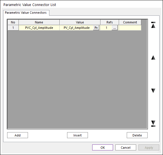
Click PV in the Value column to specify the appropriate PV.
Select PV_Cyl_Amplitude as shown below and then click OK to go return to the Parametric Value Connector List dialog box.
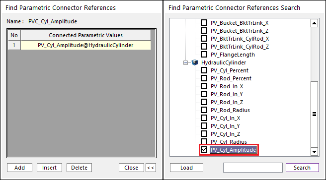
Click the More button (…) in the Refs column to display the dialog box where you will select the appropriate PV from the HydraulicCylinder subsystem. (This is similar to what you did for PPs and PPCs i n Chapter 3 of this tutorial.)
Click the Continue button (>>) next to the Close button and then scroll down to select the box next to PV_Cyl_Amplitude in the HydraulicCylinder subsystem.
Click Load to enter the appropriate values in the dialog box. Your dialog boxes should now look like the following figure.
Finish the creation process by clicking Close and then OK.
Save your model.
1.5.5. Adding a Bucket Tip Load
1.5.5.1. Task Objective
The load that you will add in this chapter represents the force at the tip of the bucket when digging. Therefore, you want the load to remain in a fixed orientation with respect to the bucket. You will accomplish this by creating an extra body (dummy body) that is fixed to the bucket (to maintain correct orientation) and applying an axial force between them that only applies force on the bucket with no reaction load on the dummy body. You will then run your first simulation of the model.
1.5.5.2. Estimated Time to Complete
15 minutes
1.5.5.3. Creating the Dummy Body
1.5.5.3.1. To create the dummy body:
From the Marker and Body group in the Professional tab, click the Ellipsoid function.
Set the Creation Method to Point, Distance.
Enter the following coordinates for the center of the sphere:
5579.2685, -207.8525, 62.560441
Enter 50 for the radius of the sphere (distance).
Zoom in on the tip of the bucket to see the sphere you created.
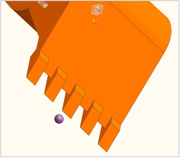
Right-click the sphere and click Properties.
In the General page, change the name of the body to BucketTip.
Click the Graphics Property page and choose Gray-50% as the color.
Click OK.
1.5.5.4. Attaching the Dummy Body to the Bucket
In this step, you will attach the dummy body to the bucket using a fixed joint.
1.5.5.4.1. To attach the dummy body to the bucket:
From the Joint group in the Professional tab, click the Fixed Joint function.
Set the Creation Method to Body, Body, Point.
Click the BucketTip and then the Bucket, and enter the following coordinates into the Input Window Toolbar:
5679.2685, -207.8525, 62.560441
This creates the fixed joint with the sphere (BucketTip body) as the Base body and the Bucket as the Action body with the joint located at the tip of the bucket where you want the load applied.
1.5.5.5. Applying an Axial Force between the Sphere and Bucket
1.5.5.5.1. To apply an axial force:
From the Force group in the Professional tab, click the Axial Force function.
Set the Creation Method to Point, Point.
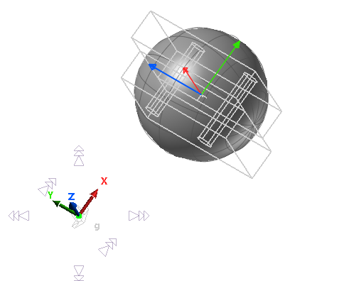
Click the center of the BucketTip and then the center of the fixed joint you just created. A close-up view of the Bucket Tip should now look like the following:
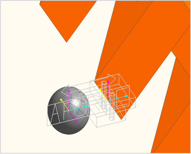
A characteristic of the axial force is that it transmits force in the z-direction of the markers at its two points. If you look closely at the model, you will see that the z-axis (yellow arrows) needs to be rotated to point in the correct direction. You also need to turn on the display of the force and make sure the force is only applied to the Action (Bucket) body. You will make these changes now.
Right-click the AFORCE icon and click Properties.
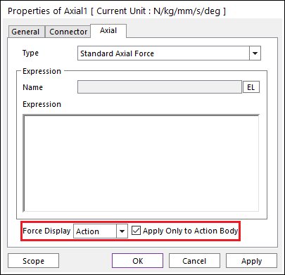
On the Axial page:
Click Apply Only to Action Body.
Set Force Display to Action as seen in the figure on the below.
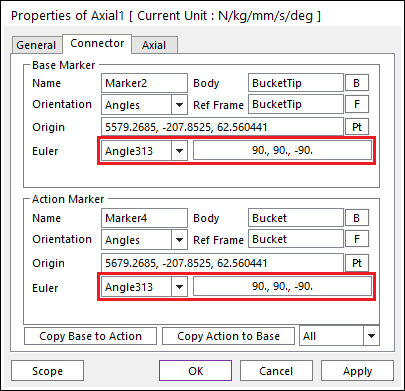
On the Connector page of this dialog box, you will rotate the markers to set their z-axes in the correct direction.
Click the Connector page and change the orientations of both markers to 90., 90., -90. as shown in the second figure on the below.
This rotates the marker 90 degrees about its +z axis, then 90 degrees about the newly positioned +x axis, then -90 degrees about the newly positioned +z axis. The result is to point the +z axis of the marker in the direction of the +x axis of the global coordinate system.
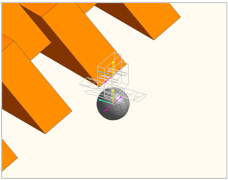
Click the General page and change the name to BucketTipLoad.
Click OK. The model should now look like the following:
1.5.5.6. Defining the Expression for the Axial Force
You will do this step a little differently than you would normally do. You will first define the expression in the Expression List and then return to the Axial Force Properties dialog box and choose the expression that you created.
1.5.5.6.1. To define the expression:
From the Expression group in the SubEntity tab, click the Expression function to open the Expression List dialog box.
Click Create.
Name the expression Ex_BucketTipLoad and enter the following function:
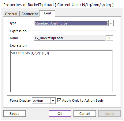
50000*IF(WZ(1,2,2):0,0,1)

This will provide a 50 kN load on the bucket tip when the rotational velocity (WZ) of the bucket is greater than zero and zero otherwise. For more information on syntax for the IF function, search for “IF Statement” in the RecurDyn Help.
The WZ function requires a marker as its argument. You write the function as WZ(1) and then define the marker Bucket.Marker1 as the first entry in the argument list as shown in the figure on the below.
To add an entity to the argument list, click Add and then either double-click the cell and type in the name Bucket.Marker1 directly or drag the marker name from the Database window and drop it in the cell (expand Bodies Bucket Markers Marker1).
Follow the same procedure to add second entity named DipperStick.Marker2.
Click OK to accept the expression and OK again to exit the Expression List dialog box.
Return to the Properties dialog box for the BucketTipLoad force.
In the Axial page, click EL and then select Ex_BucketTipLoad from the list.
Click OK. The BucketTipLoad Properties dialog box should now look like the figure on the below.
Click OK.
1.5.5.7. Running a Simulation
Now you will run a simulation of the model to verify that the force is in the correct direction.
1.5.5.7.1. To run a simulation:
From the Simulation Type group in the Analysis tab click the Dynamic / Kinematic Analysis function.
Set the following:
End time: 4.0
Step: 400
Click Simulate.
Click Play.
The following figure shows what the model should look like 1.5 seconds into the simulation.
Note in particular that the blue force vector at the tip of the bucket shows that the direction of the force is into the bucket as it should be.
1.5.6. Calculating Power Consumption
1.5.6.1. Task Objective
Tip
You can start the tutorial here using Excavator_final.rdyn, which has all the model construction completed. It is in the tutorial directory.
The design study will use the hydraulic cylinder power as a performance index (or measure). In this chapter, you will learn how to access the necessary data and how to create an expression to calculate the power used by the hydraulic cylinder. Power is the product of force and velocity.
To calculate the hydraulic cylinder power, you need to access the driving force of the translational joint in the HydraulicCylinder subsystem and pass it through to the system level. You can almost achieve this by using the reaction force of the revolute joint you just created between the dipper and the cylinder, but this value includes forces from the mass and motion of the hydraulic cylinder and so is not exact.
You will use a special technique, instead, to obtain the exact force value. You will create a dummy body in the HydraulicCylinder subsystem and apply a force to it equal in magnitude to the driving force of the translational joint. Then, you will fix this body to ground at the system level and use the reaction force in this fixed joint as the measure of the desired force.
The joint velocity will be measured from the relative velocity of the two markers defining the translational joint at the subsystem level.
1.5.6.2. Estimated Time to Complete
15 minutes
1.5.6.3. Creating the Dummy Body
First, you will create the dummy body in the HydraulicCylinder subsystem.
1.5.6.3.1. To create the dummy body:
Double-click the HydraulicCylinder subsystem in the Working model window to enter Subsystem Edit Mode.
From the Marker and Body group in the Professional tab, click the Ellipsoid function.
Set the Creation Method to Point, Distance.
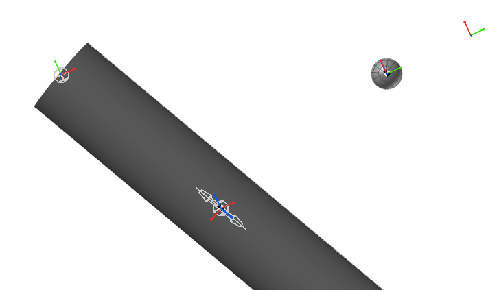
Create a sphere at the following location:
6100, -207.8525, 4200
Enter 50 in the Input Window Toolbar as the radius. The sphere appears as shown below.
Right-click the newly created body and select Properties to change the name and color of the body.
In the General page, change the name to DrivingForceBody.
In the Graphics Property page, change the color to Gray-50%.
1.5.6.4. Creating an Axial Force to Act on the DrivingForceBody
The first thing you need to do is define a marker for the reaction force on ground.
1.5.6.4.1. To create a marker:
From the Marker and Body group in the Professional tab, click the Marker function.
Set the Creation Method to Body, Point.
Click MotherBody (anywhere on the screen other than on the cylinder or rod) and then enter the following coordinates for the marker location:
6400, -207.8525, 4200
The cylinder, marker and sphere appear as shown below.
From the Force group in the Professional tab, click the Axial Force function.
Set the Creation Method to Point, Point.
Click the marker at the center of DrivingForceBody and then the newly created marker.
Right-click the axial force, and click Properties.
In the Axial page of the Properties dialog box (near the bottom), set Force Display to Base.
Tip
Because you clicked the DrivingForceBody first, it is the base body.
To define the expression for the force, click EL.
In the Expression List dialog box that appears, click Create and then:
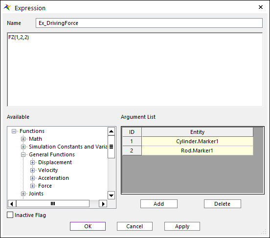
Change the name of the expression to Ex_DrivingForce.
Enter the following expression: - FZ(1,2,2)
The arguments to FZ are the markers defined in the translation joint:
Click Add under the Argument List and enter the arguments.
Cylinder.Marker1
Rod.Marker1
Tip
You can expand the list of markers under the translational joint and drag the marker names into the Argument List.
The Expression dialog box should look like the figure.
Click OK three times to accept the changes.
Click the Exit function to return to the Assembly mode.
1.5.6.5. Fixing DrivingForceBody to Ground
1.5.6.5.1. To fix DrivingForceBody to ground:
From the Joint group in the Professional tab, click the Fixed Joint function.
Set the Creation Method to Body, Body, Point.
Click ground and then, while holding down the Shift key, click DrivingForceBody from the HydraulicCylinder subsystem.
While still holding down the Shift key, click DrivingForceBody again to locate the fixed joint at the center of the body.
The orientation of the markers is important here because their orientation will be used to calculate the force in the next step.
The DrivingForceBody should look like the figure. Note that the marker’s x-axis is pointing in the global x-direction (the direction that the cylinder driving force is in).
1.5.6.6. Creating the Expression for Calculating Power
1.5.6.6.1. To create the expression:
From the Expression group in the SubEntity tab, click the Expression function to open the Expression List dialog box. Click Create in the Expression List and then the Expression window should look like the below figure.
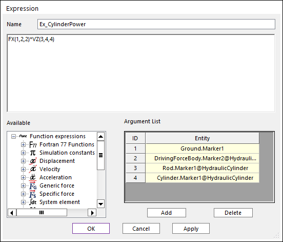
Rename the expression Ex_CylinderPower.
Enter the following expression: FX(1,2,2)*VZ(3,4,4)
Enter the four entities from the list below in that order into the Argument List:
Ground.Marker1
DrivingForceBody.Marker2@HydraulicCylinder
Rod.Marker1@HydraulicCylinder
Cylinder.Marker1@HydraulicCylinder
Click OK twice to accept the changes and close out of the Expression List.
Tip
@HydraulicCylinder in the entities names means that the specified markers are located in the HydraulicCylinder subsystem. The first two entities can be dragged and dropped from the Database window because they are the markers used in the fixed joint between DrivingForceBody and ground, but the names of the other two entities must be typed in directly because they are not accessible at assembly mode.
1.5.6.7. Creating an Output Request
In this section, you will create an expression output request so you can plot Ex_CylinderPower in the Plotting environment.
1.5.6.7.1. To create an output request:
From the Expression group in the SubEntity tab, click the Request function.
Click the Expression page, and then click Create.
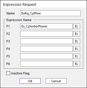
Change the name of the expression request to ExRq_CylPow.
Click EL in the F1 row and select Ex_CylinderPower from the Expression List.
Click OK. The Expression Request dialog box should now look like the one shown on the below.
Click OK twice to accept changes and close the dialog boxes.
1.5.6.8. Running a Simulation and Plotting the Results
In this step, you will verify that the expression is calculating the cylinder power correctly. If the expression is correct, there will be relatively no difference between the calculated power and the power calculated from the translational joint’s relative velocity multiplied by its driving force.
1.5.6.8.1. To run a simulation and plot the results:
Run the simulation as described previously.
Click the Plot Result function.
In the Plot Database Window, expand Joints -> TraJoint1@HydraulicCylinder.
Double-click Vel1_Relative to plot the joint velocity.
In the Plot Database Window, double-click Driving_Force.
Multiply these two curves together using the Simple Math tool:
From the Analysis Group in the Tool tab, click the Simple Math function.
Select the Multiply : F1 * F2 option in Operation Type.
Leave Source Curve1 (F1) as Vel1_Relative but change Source Curve2 (F2) to Driving_Force by selecting it from the drop-down list, as shown in the figure on the below.
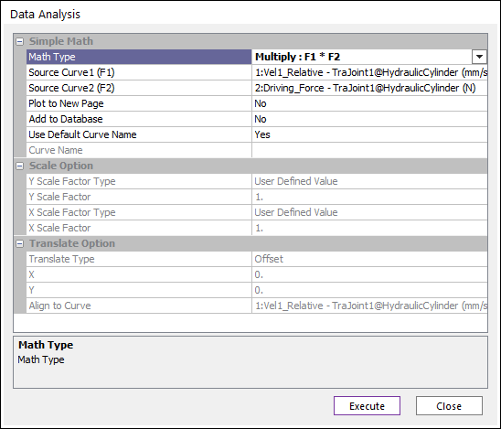
Click Execute to create the new curve.
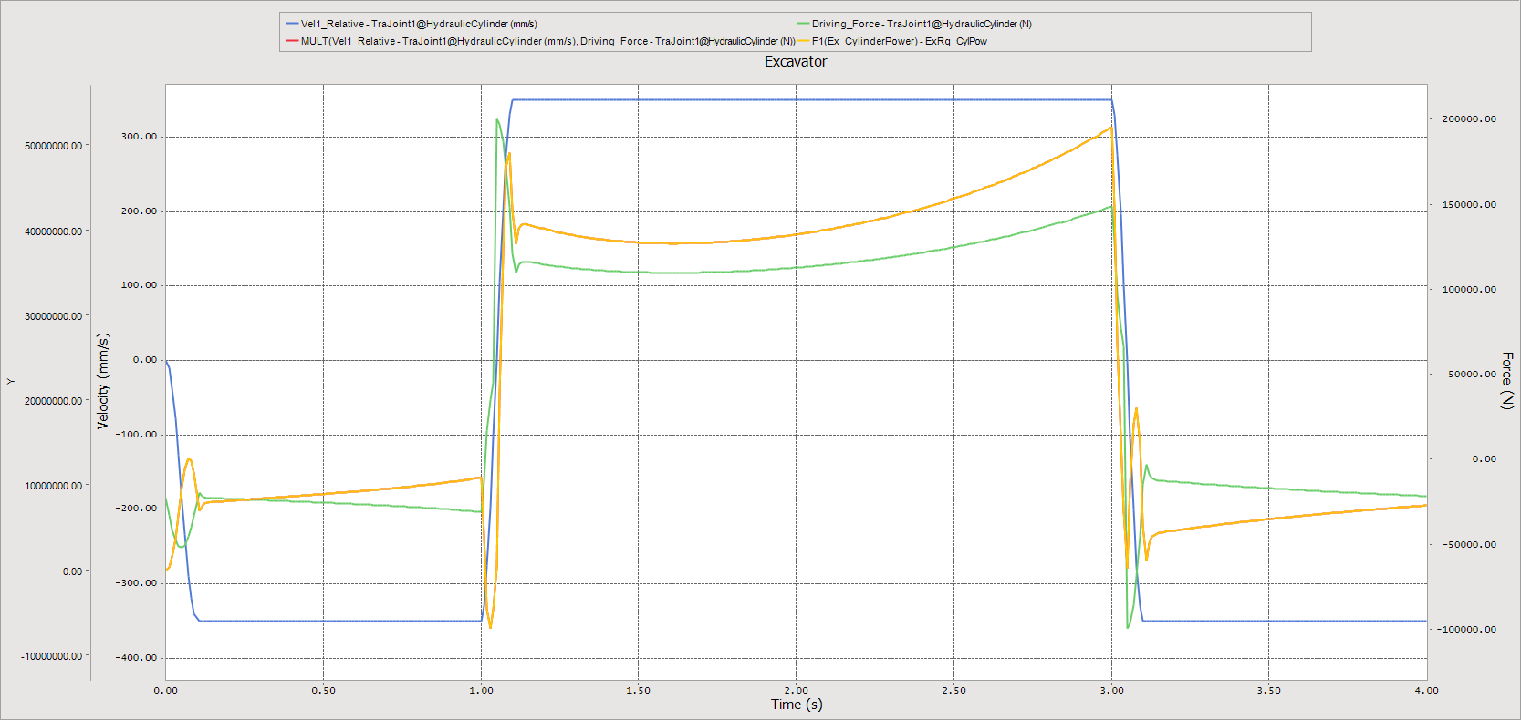
Now plot the expression for cylinder power.
In the Plot Database Window, expand Request→Expressions→ExRq_CylPow.
Double-click F1(Ex_CylinderPower). The two curves are practically identical as shown in the following figure.
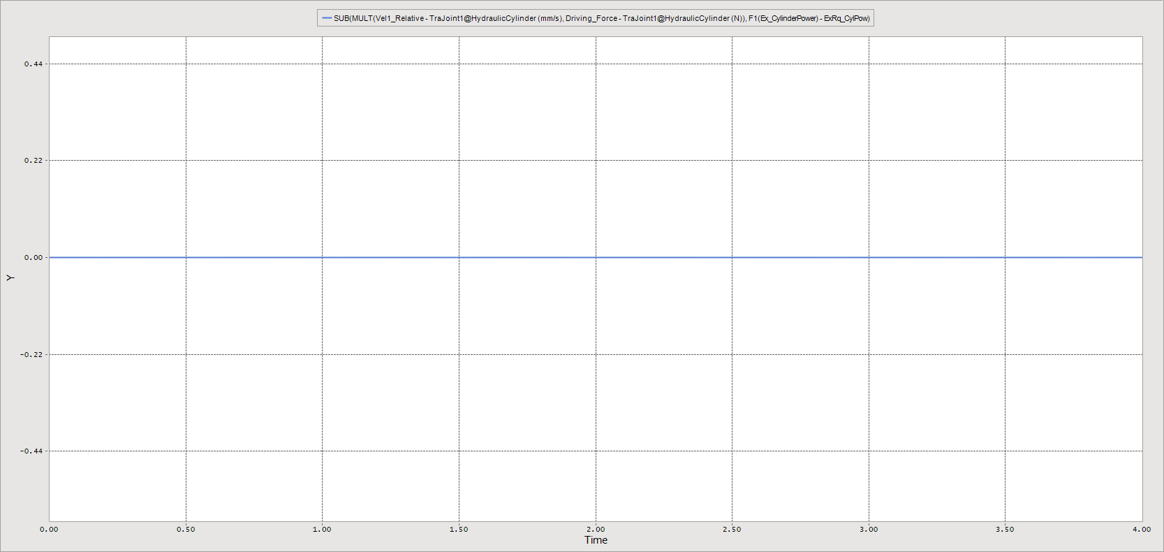
To verify that the two curves really are identical, you will calculate their difference using the Simple Math tool again.
Open the Simple Math tool as before but this time:
Change the operation to Minus: F1 – F2.
Set Source Curve1 (F1) as MULT(Vel1_Relative-TraJoint1@…),and Source Curve2 (F2) to F1(Ex_CylinderPower) by selecting it from the drop-down list, as shown in the figure on the below.
Set Plot to New Page to Yes and Execute, so you will see an uncluttered curve for the error.
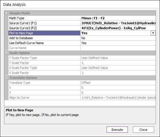
The setup of the Simple Math dialog box should look like the figure on the below.
Tip
You can change the title of the plot by right clicking to show Edit title and then changing the title text in the dialog box that appears.
1.5.7. Calculating the Range of Motion
1.5.7.1. Task Objective
In this chapter, you will create an expression that will calculate the range of motion of the bucket. This range of motion will change when you adjust the crank link length and the bucket joint angle, because these two parametric values change the geometry of the four-bar transmission at the end of the dipper. This happens even though the hydraulic cylinder length and range of travel do not change.
When you perform the design study in the next chapter, you want to include this range of motion as a performance index, so you need an expression to calculate it. The expression for finding the largest rotation in the negative direction has already been created for you. Therefore, in this chapter, you will create a similar expression for finding the largest rotation in the positive direction and then put them together to calculate the total range of motion.
1.5.7.2. Estimated Time to Complete
15 minutes
1.5.7.3. Calculating the Maximum Positive Rotation of the Bucket
In this section, you will create a new variable equation to calculate the maximum positive rotation of the bucket.
1.5.7.3.1. To calculate the rotation:
From the Equation group in the SubEntity tab, click the Variable Equation function.
In the Variable Equation List dialog box, click Create.
Change the name to VE_MaxPosRot.
In the Expression portion of the Variable Equation dialog box, click EL.
In the Expression List dialog box, click Create.
This expression needs to be able to reference itself so it can keep track of whether the current rotation is greater than previous values at each step of the simulation. Therefore, you need to enter a placeholder expression that you will then modify once you have finished creating the variable equation.
Change the name of the expression to Ex_MaxPosRot and enter the number 0 as the expression itself.
Click OK four times.
Return to the list of expressions in the Database window, and modify Ex_MaxPosRot:
Click E to change the expression to the following:
IF(VARVAL(3)-AZ(1,2):AZ(1,2),VARVAL(3),VARVAL(3))
Tip
VARVAL evaluates the variable expression in its argument, which you will set to VE_MaxPosRot in the next step. This VE, in turn, calls the expression EX_MaxPosRot, which you are currently editing. This loop means that VARVAL(3) will provide the current value of this expression. The IF statement above should be read as follows:
If the current value of this expression minus the current rotation of the bucket (VARVAL(3)-AZ(1,2)) is less than zero, then this expression equals the current bucket rotation (AZ(1,2)). Otherwise, the expression should remain unchanged.
For more information on the VARVAL and AZ functions, see the RecurDyn Help.
Now add the following three entities to the Argument List in this order:
Bucket.Marker1
DipperStick.Marker2
VE_MaxPosRot
After making these modifications the Expression dialog box should appear as follows.
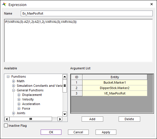
Click OK.
1.5.7.4. Calculating the Range of Motion of the Bucket
You will calculate the range of motion of the bucket by subtracting the maximum negative rotation from the maximum positive rotation. This is the same as adding their magnitudes because the negative rotation was created so it retains its negative sign. The rotation is also converted from radians to degrees.
1.5.7.4.1. To calculate the range of motion:
In the still open Expression List dialog box, click Create and set up the expression with the following characteristics:
Name: Ex_RangeOfMotion
Expression: 180*(VARVAL(1)-VARVAL(2))/PI
Entities: VE_MaxPosRot and VE_MaxNegRot
The Expression dialog box should appear as shown on the below.
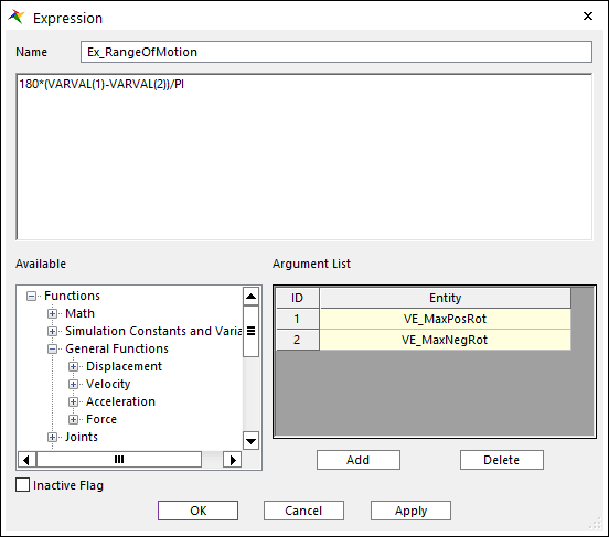
Click OK twice to exit.
1.5.7.5. Adding the New Expression to the Request
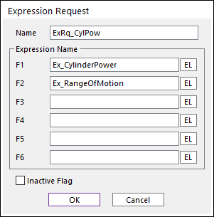
1.5.7.5.1. To add the new expression:
In the Plot Database Window, double-click the request ExRq_CylPow.
In the Request List dialog box, click Rq to modify the request.
Click EL in the F2 row.
Select Ex_RangeOfMotion from the Expression List dialog box.
Click OK three times to exit.
The Expression Request dialog box should look like the figure shown on the below.
1.5.7.6. Plotting the Expression to Verify Results
1.5.7.6.1. To plot the results:
Run the simulation as before. (Tip: End time: 4, Step: 400)
Click the Plot Result function to open the plotting environment.
To plot the rotation of the bucket joint, in the Plot Database window, expand Joints -> Rev_Dipper_Bucket, double-click Pos1_Relative.
To plot Ex_RangeOfMotion, in the Plot Database window, expand Request -> Expressions -> ExRq_CylPow and double-click F2(Ex_RangeOfMotion).
The next figure shows the desired plot.
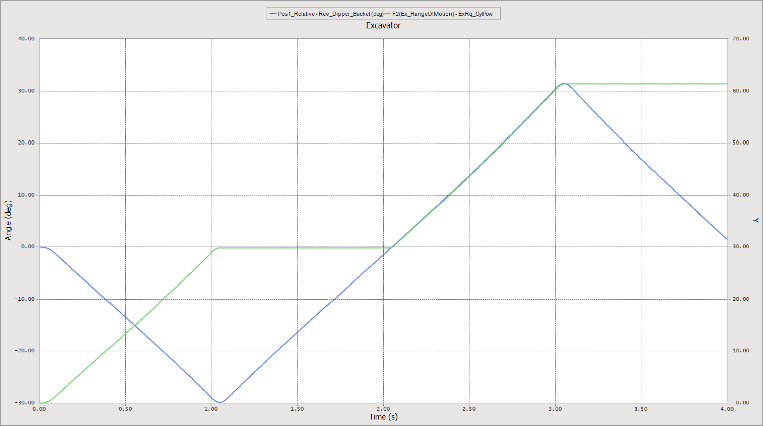
A visual inspection of the curves indicates that the function is working correctly, but to view a numerical comparison, uses the Trace Data function.
Click the Trace Data function of the Tools group in the Home tab and scroll around the two curves. Placing the cursor on the expression’s curve shows that the maximum value is 61.34 degrees. Placing the cursor on the red curve shows the following.
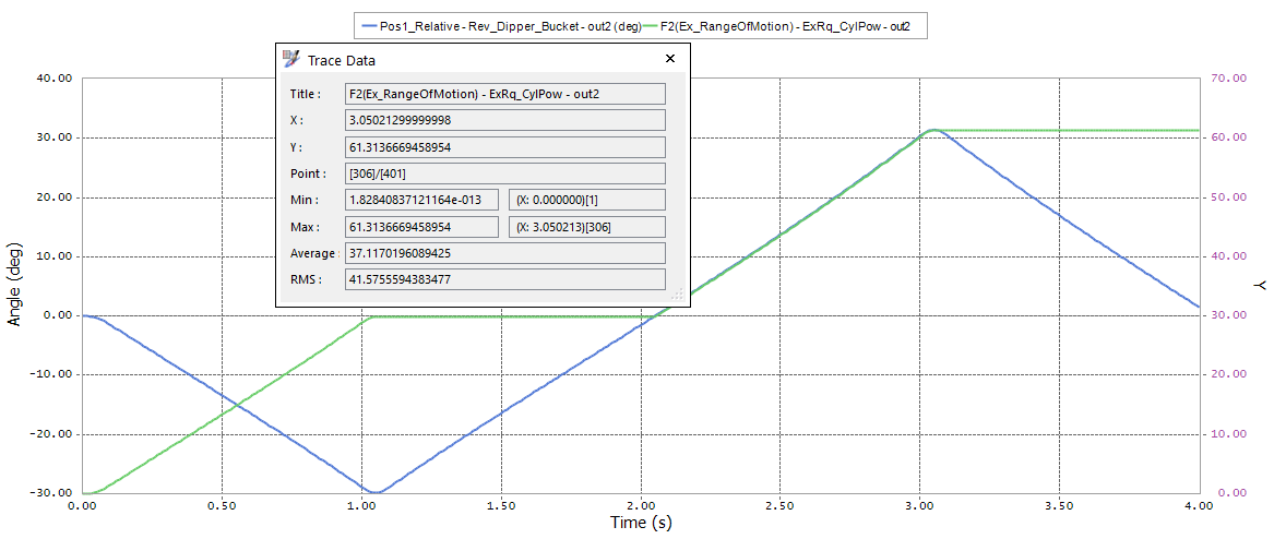
The maximum rotation is 31.47 and the minimum is -29.84 so the range of motion should be 31.47 deg - (-29.84 deg) = 61.31 deg. The small difference is explainable because the expression evaluates every single point in the entire simulation while the plot only provides the requested number of data points (400 in this case). The bucket must have rotated just a little bit farther than what is reported in the plot data.
Return to the modeling window. (File > Close)
Save your model.
1.5.8. Running and Analyzing a DOE
1.5.8.1. Task Objective
In this chapter, you will set up and run a design study to look at the effects of the crank length and bucket joint angle on the range of motion and cylinder power as defined previously. You will run a design of experiments with three levels for each variable and then look at the results.
1.5.8.2. Estimated Time to Complete
15 minutes
1.5.8.3. Setting Up the Design Variables
1.5.8.3.1. To set up the design variables:
Click the Design Variable function from the Design Study group in the Subentity tab.
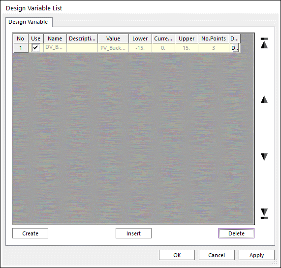
The Design Variable List dialog box appears as shown on the below. Note that the bucket joint angle is already defined as a design variable.
In the Design Variable List dialog box, click Create.
In the Design Variable dialog box that appears, change the name of the design variable to DV_DeltaCrankLength.
Click PV next to the Value text box and then select PV_DeltaCrankLength from the Parametric Value List dialog box.
Click OK.
In the Design Variable dialog box, set Value Range to Absolute Min and Max Value.
Set Min Value to -150.0 and Max Value to 150.0 as shown in the following dialog box.
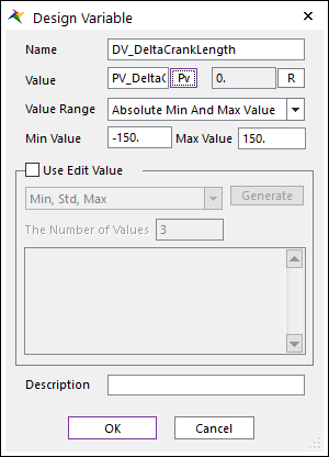
Click OK twice to accept settings and close the dialog boxes.
1.5.8.4. Defining the Performance Indexes
1.5.8.4.1. To define the performance indexes:
Click the Performance Index function from the Design Study group in the Subentity tab. The Performance Index List dialog appears.
Set the Type at the bottom left to Expression and Click the Add button in the Performance Index List window. In the Performance Index - Expression dialog Change:
Name: PI_RMSCylPower
Result Output: Ex_CylinderPower (Click EL, select the expression, click OK)
Treatment: RMS Value
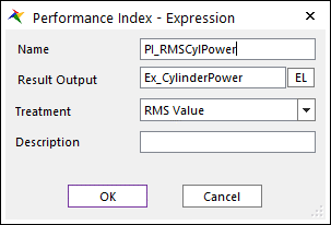
Click OK.
Click Add to add another Performance Index:
Name: PI_RangeOfMotion
Result Output: Ex_RangeOfMotion
Treatment: End Value
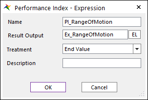
Click OK.
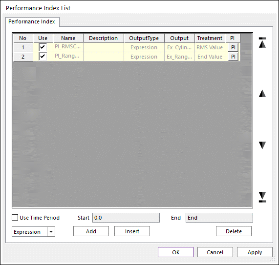
The Performance Index List now appears shown on the below.
Click OK.
1.5.8.5. Running the DOE
1.5.8.5.1. To run the design study:
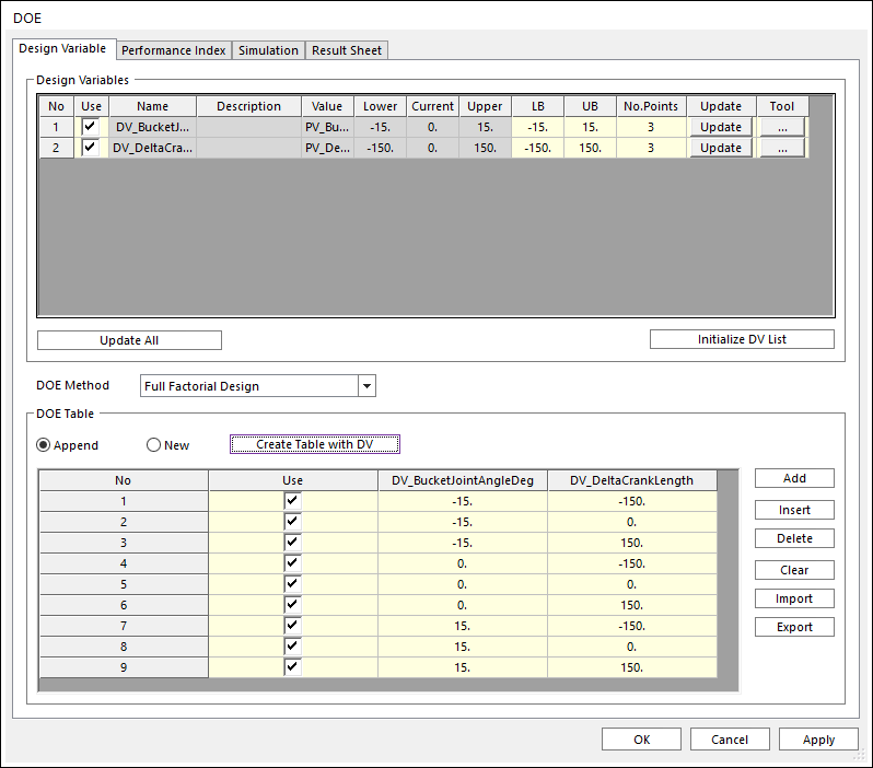
Click the Design Study function from the Simulation Type group in the Analysis tab. The DOE window appears.
Change 3 in Number of Points of DV_BucketJointAngleDeg and click the Update.
Also, change 3 in Number of Points of DV_DeltaCrankLength and click the Update.
Select DOE Method as Full-Factorial Design.
Click the Create Table with DV button and you will see 9 Trials created as shown below.
In the DOE dialog, click the Simulation page.
Click to R-Button in Number of Trials and you can see that it is updated to 9.
Click Simulate.
When the study is finished, click Result Sheet page in the DOE dialog.
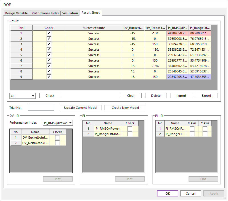
In the Result Sheet, you can see the minimum and maximum values, respectively, of each variable or result. The results for this study show that to obtain a reduction in the RMS cylinder power, you need to forfeit range of motion. This is quite reasonable when considered in terms of mechanical and geometric advantage. If you change the four-bar linkage so the mechanical advantage increases, you will be able to decrease the amount of force required from the actuator to resist a constant load at the bucket tip.
But an increase in mechanical advantage means that the geometric advantage will decrease. That is, the same actuator displacement will result in a smaller output displacement, and the result is a smaller range of motion. There is a fundamental trade-off between the range of motion and the actuator force (which affects the actuator power).
1.5.9. Running the Simulation in Batch Mode
1.5.9.1. Task Objective
In this chapter, you will set up three simulations that will run in batch mode. The simulations you will set up correspond to trials 5, 6, and 7 that were performed in the Design Study. You will then plot the hydraulic cylinder power and bucket motion.
Note that the results will be the same as the results from the design study, but there is an important reason to learn how to run batch simulations. The design study automates the running of a set of trials; however, the limitation is that only one design study can be run at a time. In batch mode, however, there is no limit to the number of simulations that can be run. For this reason, running RecurDyn in the batch mode is a good way to take advantage of nights and weekends.
1.5.9.2. Estimated Time to Complete
15 minutes
1.5.9.3. Setting up and Exporting the RecurDyn Design Parameter File
First, you need to tell RecurDyn which points, and values will be in the design parameters used in the batch simulations. This model only uses two parametric values (PVs) to make changes to the model, so you will use them here. Parametric points could just as easily be used in batch simulations, however, and the procedure is the same.
The one limitation to keep in mind is that only parametric points and parametric values at the main system level can be used. If parametric points or values are located in subsystems, they must first be set up at the main level and synchronized with parametric point connectors (PPCs) and parametric value connectors (PVCs) as discussed previously in this tutorial.
1.5.9.3.1. To set up and export the file:
In the Database window, double-click any PV to open the Parametric Value List.
Check the boxes in the DP column for PV_DeltaCrankLength and PV_BucketJointAngleDeg as shown in the figure on the below.
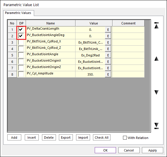
Click OK.
From the File menu, click the Export function.
Set the Files of type to RecurDyn Design Parameter File (*.rdp).
Set the export directory where RecurDyn Model file is located.
Name the file Excavator.rdp and click Save.
This creates a number of files in your working directory. The RDP file is the database that tells RecurDyn where to find PVs and PPs during the batch simulations. You should also notice that. rpp and .rpv files were created for the main system and each subsystem that contains PPs and PVs. Because you have only defined two PVs at the system level, the only file with any information in it should be Excavator.rpv. The contents appear as follows when opened in Notepad:
!=========================RecurDyn Parametric Value===================\|
PV_DeltaCrankLength = 0.
PV_BucketJointAngleDeg = 0.
This means that the current values for these design parameters are zero. When you write the batch file in the following steps, you will tell it to change these values and RecurDyn will update them automatically.
1.5.9.4. Setting Up and Exporting the RecurDyn Scenario File
The RecurDyn Scenario File (.RSS) tells RecurDyn how to run the simulation in batch mode. First, you will specify which integrator to use and then specify the simulation settings, including the simulation time and number of steps.
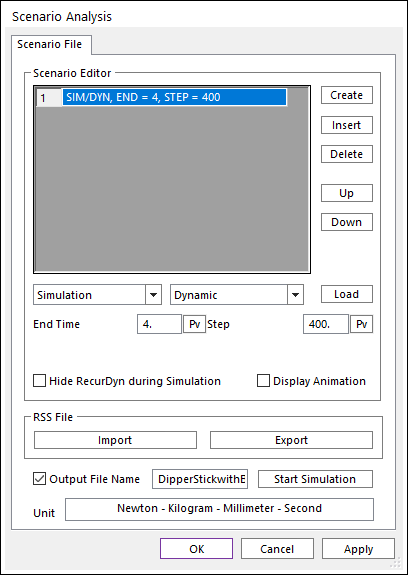
1.5.9.4.1. To set up and export the scenario file:
From the Simulation Type group in the Analysis tab, click the Scenario Analysis function.
In the Scenario Analysis dialog box, click Create.
Set up the simulation settings:
Click Create again to create a new row in the Scenario Editor.
Change the left-most drop-down box to Simulation.
Change the Endtime to 4 and the Steps to 400.
Click Load.
Your window should now look like the below.
With the settings set, you will now test the scenario.
1.5.9.4.2. To test the scenario:
Click Start Simulation.
It runs the same simulation as in the last section.
In the Scenario Analysis dialog box, click Export.
Save the file as Excavator.rss (where RecurDyn Model file is located). Open the contents of the file, in a text editor, such as Notepad. It looks like the following:
SIM/DYN, END = 4, STEP = 400
STOP
1.5.9.5. Creating the Batch File and Running the Simulation
Now you will create the batch file.
1.5.9.5.1. To create the batch file:
Open a text editor, such as Notepad, and enter the following text:
mkdir out
“<InstallDir>\Help\DP_Study\ConvertDP.exe” /clean /convert Excavator.rdp PV_DeltaCrankLength=0 PV_BucketJointAngleDeg=0
“<InstallDir>\Bin\RecurDyn.exe” “Excavator.rdyn” /rdp Excavator.rdp /rss Excavator.rss /out out\out1
“<InstallDir>\Help\DP_Study\ConvertDP.exe” /clean /convert Excavator.rdp PV_DeltaCrankLength=150 PV_BucketJointAngleDeg=0
“<InstallDir>\Bin\RecurDyn.exe” “Excavator.rdyn” /rdp Excavator.rdp /rss Excavator.rss /out out\out2
“<InstallDir>\Help\DP_Study\ConvertDP.exe” /clean /convert Excavator.rdp PV_DeltaCrankLength=-150 PV_BucketJointAngleDeg=15
“<InstallDir>\Bin\RecurDyn.exe” “Excavator.rdyn” /rdp Excavator.rdp /rss Excavator.rss /out out\out3
Note that you can directly copy the above text in the batch file if you have access to the digital form of this tutorial document.
Now save the file as Excavator.bat and close it. The following is a brief description of what each command means and does:
mkdir out
Creates a directory named out in your working directory. This is where RecurDyn will store the results of the simulations.
“<InstallDir>\Help\DP_Study\ConvertDP.exe”
Runs the ConvertDP executable file, which is in the standard RecurDyn installation in the Help>DP_Study folder. If your installation directory is different than that specified above, you will need to change this line appropriately.
/clean /convert Excavator.rdp PV_DeltaCrankLength=0 PV_BucketJointAngleDeg=0
These are the arguments to the ConvertDP executable. They tell RecurDyn to use the Excavator.rdp file and set the value of PV_DeltaCrankLength to 0 and PV_BucketJointAngleDeg to 0. Because these are already the default values, they are not really necessary but are included to show the pattern.
“<InstallDir>\Bin\RecurDyn.exe”
This provides the full path to the RecurDyn program. This should be the default for the version 8.1 installation, but if you are running a different version or specified a different location for the program, you should update your text appropriately.
“Excavator.rdyn”
Tells RecurDyn which model (.rdyn) file to use for the simulations. If you have renamed your file when saving, you should update this text accordingly. Moreover the batch file you just created should be located as same folder as Excavator.rdyn file saved, or else you must set full directory as following.
/rdp Excavator.rdp /rss Excavator.rss
Defines the file names for the .RDP and .RSS files you created earlier.
/out out\out1
Tells RecurDyn to store the output files in the out folder you created in the first line of the batch file and with the filename out1. In this case, uncheck the Create Output Folder of the Simulation Model Setting group in the Home tab.
The remainder of the batch (.bat) file contains three repetitions of the same code except the PVs are set to the values from configurations 6 and 7 in the design study you performed and the output files are named out2 and out3, respectively.
To run the simulation, first close your model in RecurDyn. You do not need to exit RecurDyn, but the batch simulation cannot run if the model it is trying to update and simulate is already open.
Double-click the Excavator.bat file you just created.
After double-clicking the file, a DOS command prompt opens and the first five lines (three commands: mkdir, ConvertDP.exe, and RecurDyn.exe) of code appear. RecurDyn opens, runs the simulation, and then closes.
The next ConvertDP.exe and RecurDyn.exe appear, and RecurDyn runs and closes again, and then once again.
1.5.9.6. Plotting the Results
1.5.9.6.1. To plot the results:
Open your RecurDyn model again and click on the Plot Result function to enter the plotting environment.
From the File menu, click the Import function and then click Import File.
Double-click the out folder and then select all three output files.
Tip
You can do this easily by first clicking out3.rplt and then, while holding down Shift key, clicking out1.rplt.
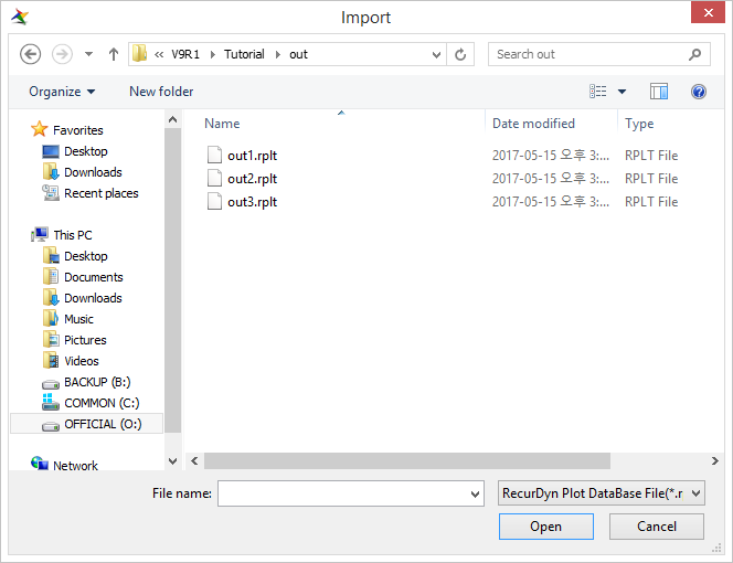
Click Open.
Now you will plot the bucket rotation and hydraulic cylinder power for all three configurations.
In the Plot Database window, expand Joints -> Rev_Dipper_Bucket right-click Pos1_Relative, and select Multi Draw.
Three curves are added to the plot. Note that, depending on how you selected the RecurDyn Plot database files in Step 3, out1, out2, and out3 may be in a different order in the Plot Database window.
Your plot window appears as shown next.
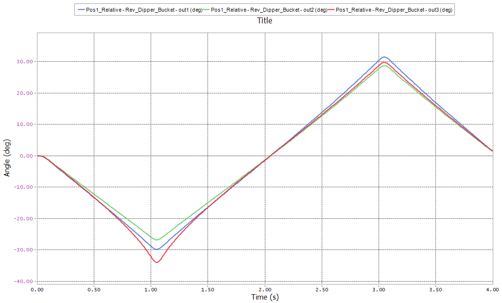
This plot shows that the first (default) configuration has the largest positive rotation, but the third one has the largest negative rotation, giving it the largest range of motion (as you discovered earlier in the Design Study). The second configuration has about the same positive rotation as the third, but it has significantly smaller negative rotation giving it the smallest range of motion.
Click Show Left Windows of the View group to open a new plot window.
Click the lower plot anywhere in the window to activate it.
In the Plot Database Window, expand Request -> Expressions -> ExRq_CylPow and right-click F1(Ex_CylinderPower), and select Multi Draw.
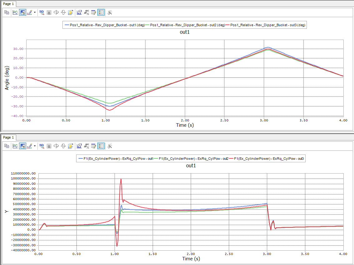
From this plot, you see that the power for the third configuration is very large at the point of maximum negative rotation. This is indicative of a poor mechanical advantage, meaning that a large input (hydraulic cylinder) force is required to sustain a significantly smaller output force (bucket tip load). Because a poor mechanical advantage corresponds to a good geometric advantage, it makes sense that at that point in the simulation the third configuration has a larger rotation of the bucket than the other configurations for the same input displacement.
If you would like, you can change the titles, axis labels, and legend entries for the plots so they look like the final versions shown on the next page and on the first page of the tutorial.
1.5.9.6.2. To change a title or axis label:
Double-click the title or axis label.
Enter new text.
1.5.9.6.3. To change the legend:
Double-click the legend.
Click Change Name.
You can reposition any of the above items by simply clicking and dragging