7.1. Compliant Clutch Tutorial (FFlex)

7.1.1. Getting Started

7.1.1.1. Objective

The modeling and simulation of contact between flexible bodies is an important topic in multibody dynamics. The RecurDyn FFlex toolkit has powerful capabilities to define and simulate flexible bodies that have sliding or rolling contact with other bodies.

The example in this tutorial is a centrifugal clutch for a snowmobile, which relies on a compliant, or flexible, plate to operate. The benefits of using a compliant clutch plate, as opposed to having separate moving parts with springs, is that the part count is greatly reduced. This simplifies the manufacturing process and increases the reliability of the mechanism, as well.

Note that the model used in this tutorial is not based on any actual product or design concept but borrows from suggested applications for compliant mechanisms published by the Brigham Young University Compliant Mechanisms Research Center.

7.1.1.2. Audience

This tutorial is intended for new users of RecurDyn who have previously learned how to create geometry, joints, force entities, and 2D contacts. All new tasks are explained carefully.

7.1.1.3. Prerequisites

Users should first work through the 3D Crank-Slider, Engine with Propeller, and Pinball (2D contact) tutorials, or the equivalent. We assume that you have a basic knowledge of physics.

7.1.1.4. Procedures

The tutorial is comprised of the following procedures. The estimated time to complete each procedure is shown in the table.

Procedures	Time (minutes)
Importing the model geometry	10
Adding joints and forces	15
Defining surfaces and contacts	20
Creating a boundary condition	5
Simulating the model	15
Total	65

7.1.1.5. Estimated Time to Complete

65 minutes

7.1.2. Importing the Model Geometry

7.1.2.1. Task Objective

Learn how to import both rigid and flexible bodies to create the compliant clutch model.

7.1.2.2. Estimated Time to Complete

10 minutes

7.1.2.3. The Compliant Clutch Model

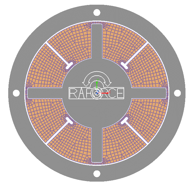
The model being used in this tutorial is a centrifugal clutch that relies on the flexibility of the clutch plate to operate. The following is a diagram of the clutch.

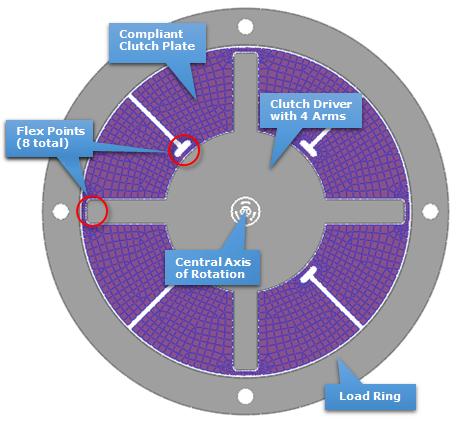
When power source rotates the clutch, driver is about the central axis, the arms push the compliant clutch plate into rotation, as well. As the rotational speed increases, centrifugal force pulls the clutch plate radially outwards, which flexes at eight flex points. As the plate moves outwards, it comes into contact with the outer ring to which the load is connected. Friction between the clutch plate and the load ring causes the load ring to begin to rotate, thereby transferring power from the clutch driver to the load.

In the RecurDyn model you will be creating, the compliant clutch plate will be treated as a flexible body, and a NASTRAN bulk data file will be imported for this part. The other bodies will be treated as rigid bodies, and geometry files will be imported for these parts.

Note

To make the simulation more efficient for the tutorial, the model represents a 1 mm thick cross section of what the actual clutch would be. Driving and load torques have been scaled appropriately, and the same treatment can be applied to the simulation results you will obtain when interpreting them.

7.1.2.4. Starting RecurDyn

7.1.2.4.1. To start RecurDyn and create a new model:

1. On your Desktop, double-click the RecurDyn tool. RecurDyn starts and the New Model window appears.

2. Enter the name of the new model as FFlexClutch.

   

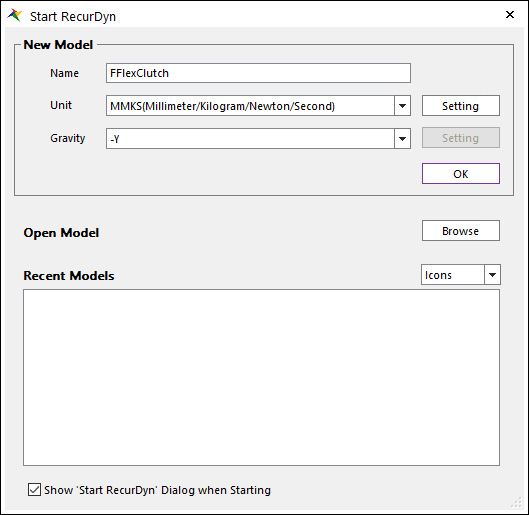
3. Click OK.

7.1.2.5. Importing the Compliant Clutch Plate Mesh Data

Now you will import the mesh data for the clutch plate into the model. In this case, the geometry was modeled in the CAD system in the correct locations. You do not need to adjust the geometry position.

7.1.2.5.1. To import a mesh data file:

1. From the FFlex group in the Flexible tab, click the Import FFlex Body function.

2. Select the point (0, 0, 0) as the origin by doing one of the following:

   • In the Input Window Toolbar, enter 0, 0, 0.

   • In the Working Window, select the point.

3. Select the clutchPlate.dat.

   (The file path: <InstallDir>\Help\Tutorial\Flexible\FFlex\CompliantClutch)

4. Click Open.

5. In the Import dialog box that appears, change Body Name to FFlexClutchPlate.

   

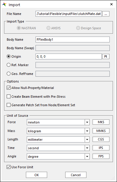
6. Click OK. The clutch plate appears in the Working window but is small.

7. Fit the geometry to the window by pressing F key, and change the grid spacing, icon size, and marker size to 10.

   The model appears as shown next.

   

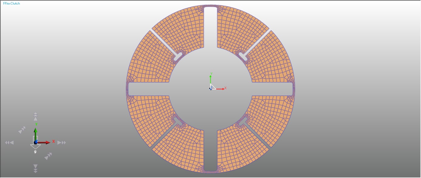
8. Change rendering mode to Shade.

7.1.2.6. Importing the Rigid Geometry

7.1.2.6.1. To import the driver:

1. From the File menu, click the Import function.

2. Set Files of type to ParaSolid File (*.x_t,*.x_b …).

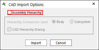
3. In the FFlex tutorial folder, select the file: clutchDriver.x_t.

   (The file path: <InstallDir>\Help\Tutorial\Flexible\FFlex\CompliantClutch)

4. Click Open. The CAD Import Options window appears. Clear the Assembly Hierarchy checkbox and click Import.

   

5. In the Database Window, right-click ImportedBody1, and click Properties.

6. On the General page, rename the body ClutchDriver.

7. Click OK.

7.1.2.6.2. To import the load ring:

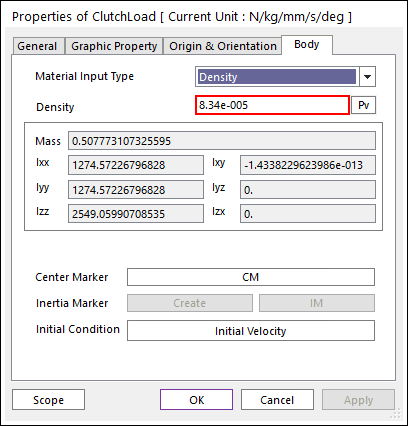
1. Repeat steps 1 through 7 above, this time importing the file clutchLoad.x_t, and naming the body ClutchLoad.

   (The file path: <InstallDir>\Help\Tutorial\Flexible\FFlex\CompliantClutch)

2. Click the Body page.

3. In the Density text box, enter 8.34e-05.

   This increases the rotational inertia of the load, simulating the weight of the snowmobile.

   

At this point, all the components of the clutch are present, but the rendering of the circular edges is poor. You will now improve the quality of the rendering, which will be important later when viewing the surface contact interactions in the animations.

7.1.2.6.3. To improve the rendering of the geometry:

1. From the Setting group in the Home tab, click the Display Setting function.

2. Select the Geometry page.

3. Move the sliders next to Curve Detail Level and Geometry Detail Level to High.

   

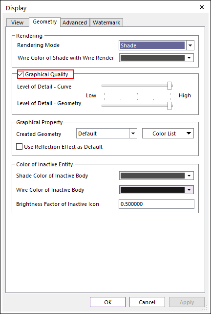
4. Click OK.

7.1.2.6.4. Save the model

7.1.3. Adding Joints and Forces

You will now add revolute joints, as well as driving and load torques, to the model.

7.1.3.1. Task Objective

Learn to:

• Create revolute joints.

• Create expressions, which will be used to create driving and load torques.

7.1.3.2. Estimated Time to Complete

15 minutes

7.1.3.3. Creating Revolute Joints

Now you will create two revolute joints, one for the driver and one for the load. The clutch plate will be constrained by the other geometry, so no joint must be added for that body.

7.1.3.3.1. To create the driver joint:

1. From the Joint group in the Professional tab, click the Revolute Joint function.

2. Set the Creation Method to Body, Body, Point.

3. Click anywhere in the background of the Working Window (not on any bodies) to select Ground as the first body.

4. Click the ClutchDriver body to select it as the second body.

5. In the Input Window Toolbar, enter 0, 0, 0 as the joint location.

6. In the Database Window, right-click RevJoint1, and click Properties.

7. On the General page, rename the joint Rev_driver.

8. Click OK.

You will create the revolute joint for the clutch load in a similar way, but you will add friction.

7.1.3.3.2. To create the load joint:

1. Click the Revolute Joint function again. Ensure that the creation method is still Body, Body, Point.

2. Click anywhere in the background of the Working window to select Ground as the first body.

3. Click the ClutchLoad body to select it as the second body.

4. In the Input Window Toolbar, enter 0, 0, 0 as the joint location.

5. In the Database window, right-click RevJoint1, and click Properties.

6. On the General page, rename the joint Rev_load.

7. Click the Joint page.

8. Click the checkbox next to Include Friction and click Sliding & Stiction.

9. Make the following changes to the settings:

   • Static Friction Coefficient: 0.1

   • Dynamic Friction Coefficient: 0.1

   • Effect - Stiction: uncheck

   • Friction Arm: 20

   • Pin Radius: 20

   • Bending Moment: uncheck

     

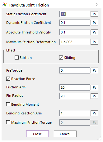
10. Click Close.

11. Click OK.

7.1.3.4. Creating the Torque Expressions

You will now create expressions for the driving and load torques:

• The driving torque will be a stepped transition from 0 to 10,000 N∙mm over 0.01 seconds.

• The load torque will be in the opposite direction of the driving torque, and will vary with the load’s rotational velocity, squared. This simulates the load that a snowmobile would experience due to wind resistance.

As stated earlier, the torques have been scaled down to match the model.

7.1.3.4.1. To create the driving torque expression:

1. From the Expression group in the SubEntity tab, click the Expression function.

2. Click Create. Refer to the following diagram for the next several steps.

   

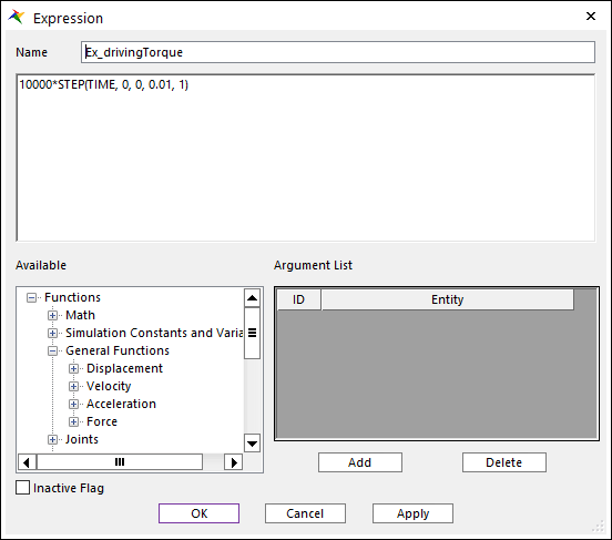
3. Change the name to Ex_drivingTorque.

4. For the expression, enter: 10000*STEP(TIME, 0, 0, 0.01, 1).

5. Click OK.

7.1.3.4.2. To create the load torque expression:

1. Click Create to create a new expression. Refer to the diagram below for the next several steps.

   

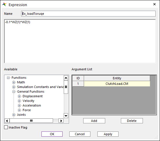
2. Name the expression Ex_loadTorque.

3. For the expression, enter: -0.1*WZ(1)*WZ(1).

4. Under Argument List, click Add.

5. In the Database Window, expand Bodies > ClutchLoad > Markers > CM.

6. Click and drag CM to the empty box under Entity, to enter it as the first argument.

7. Click OK twice.

7.1.3.5. Creating the Driving and Load Torques

You will create driving and load torques to the clutch driver and load at the revolute joints and link them to the expressions you just created.

7.1.3.5.1. To create the driver torque:

1. From the Force group in the Professional tab, click the Rotational Axial Force function.

2. Set the Creation Method to Joint.

3. In the Working Window, right-click near the two revolute joints, and click Select List.

   

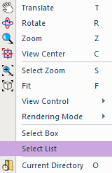
   A list of entities that are able to be selected at that screen location appears.

4. From the list, select Rev_driver.

   

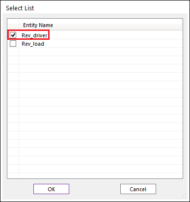
5. Click OK.

6. In the Database Window, right-click RotationalAxial1 (under Forces) and click Properties.

7. Click EL.

8. From the Expression List window, select Ex_drivingTorque.

9. Click OK. The Properties dialog should now appear as shown at below.

   

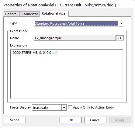
10. On the General page, rename the force RotAx_driver.

11. Click OK.

After creating the driving torque, the model appears as shown below:

7.1.3.5.2. To create the load torque:

Repeat the steps above, this time:

• Selecting Rev_load as the joint.

• Selecting Ex_loadTorque as the expression.

• Renaming the force RotAx_load.

7.1.3.5.3. Save the model

7.1.4. Defining Surfaces and Contacts

In this chapter, you will create the necessary entities for a flexible surface to rigid surface contact.

7.1.4.1. Task Objective

You will:

• Create a contact surface on a flexible body.

• Define a contact between the flexible surface and a rigid surface.

7.1.4.2. Estimated Time to Complete

20 minutes

7.1.4.3. Contacts in the Model

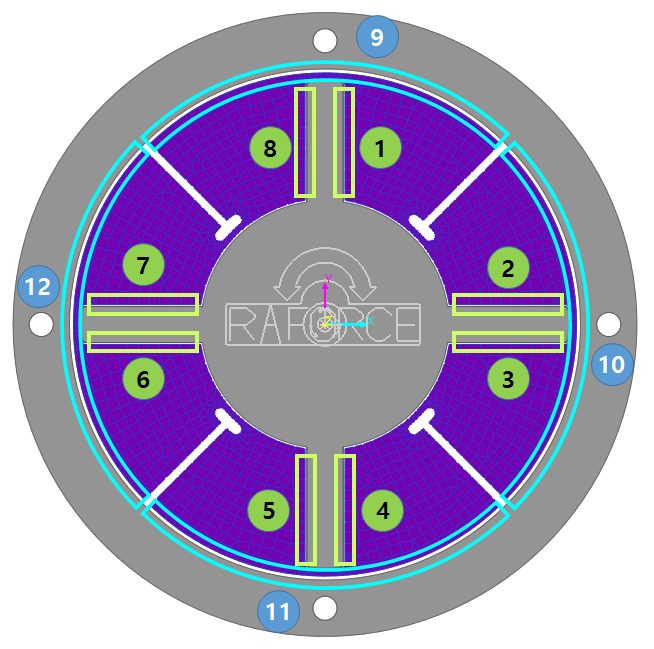
You will now create 12 contacts in the model, each representing the interaction between two surfaces. In this model, some contacts will be between surfaces on the driver and the plate, and others between the plate and the load.

• If the contact surface is on the plate, it is defined by selecting a set of element faces from the finite element mesh. This set of element faces is referred to as a Patch Set.

• If the contact surface is on the driver, it is defined as a face surface.

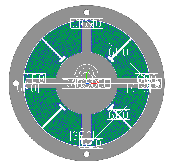
The figure below shows the 12 regions where the contacts will be created, and the numbering scheme that will be used in the rest of the tutorial.

7.1.4.3.1. Contact Layout Diagram

Note

Not all of the possible contact regions in the clutch have been selected to be modeled. This is because when the driver rotates the clutch plate, centrifugal force will pull the plate elements outwards, towards the clutch load. With this in mind, you can reduce the number of contacts and, therefore, reduce the simulation time.

7.1.4.4. Creating the Patch Sets

As explained before, if the surface is on the plate, you need to create a patch set before defining the contacts. There are nine patch sets that you need to create. To make it easy for you, after creating the first patch set, you can open an intermediate model that contains the patch sets already defined. If you would like more experience creating the patch sets, follow the instructions in Appendix A, Creating the Remaining Patch Sets, on page 47.

7.1.4.4.1. To create a patch set on a flexible body:

1. In the Database Window, right-click FFlexClutchPlate, and click Edit.

   RecurDyn is now in Body Edit Mode for the clutch plate.

2. From the Set group in the FFlex Edit tab, click the Patch Set function.

3. Select red, as shown at below.

   

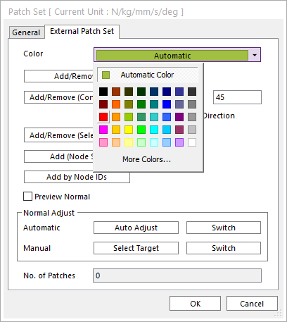
4. Change Tolerance (Degree) to 20.

5. Click Add/Remove (Continuous).

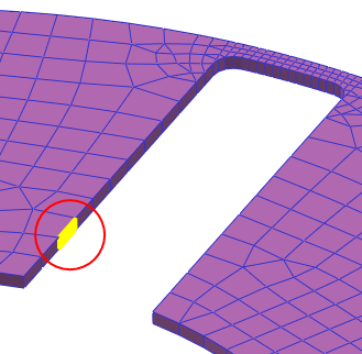
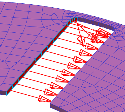
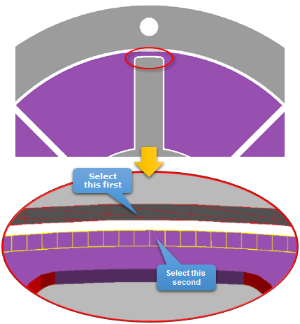
6. Zoom in carefully to the FFlexClutchPlate geometry as shown in the figure at below and select the element as shown at below, highlighted in light yellow.

   

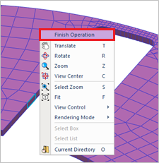
7. In the Working Window, right-click, and click Finish Operation.

   

8. Click Add/Remove in the patch set dialog.

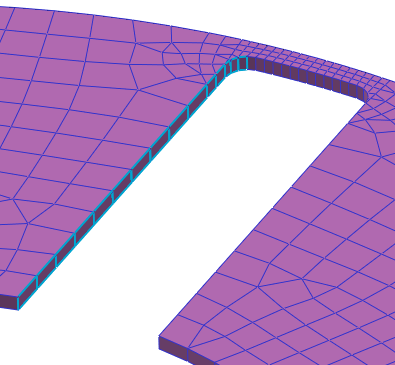
9. Holding down the Ctrl key, select the element faces of the first contact surface, as shown at below, highlighted in sky blue and right-click, and click Finish Operation.

   

   Tip

   How to select faces easily:

   To deselect elements which you mistakenly selected, continue to hold the Ctrl key and click again on the same element. It will toggle between being selected and deselected. In the current selection mode, if you forget to hold the Ctrl key down and select another element, all the previously selected elements will be deselected and only the element you just clicked on will be selected.

   - Select Add from the Flexible Toolbar, as shown below.

   

   - Also note that there is a Remove option. Selecting this will change the selection behavior so that elements are only deselected when clicked on.

10. In the patch set dialog, click the checkbox next to Preview Normal.

11. Ensure that all the normals are pointing out from the surface, as shown in the figure on the below. If not, click Auto Adjust (to the right of Automatic) to switch all of the normals to be consistently oriented in the same direction. If that direction is not the desired direction, click Switch to switch the normals.

    

12. Click OK.

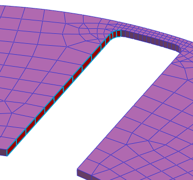
13. The patch set should now appear in red as shown at below.

    

7.1.4.4.2. At this point, you can either:

• Open the intermediate model, FFlexClutch_Intermediate.rdyn, with the remaining patch sets already defined and continue with the next section, Creating the Face Surfaces.

  (The file path: <InstallDir>\Help\Tutorial\Flexible\FFlex\CompliantClutch)

• (OR, Follow the instructions in Appendix A, Creating the Remaining Patch Sets, to define the remaining patch sets yourself to gain experience.)

7.1.4.4.3. Save the model

• If you use FFlexClutch_Intermediate.rdyn model, Save as other path because you cannot simulation this model in install path.

7.1.4.5. Creating the Face Surfaces

7.1.4.5.1. To create a face surface on a rigid body:

1. In the Database window, right-click ClutchDriver, and click Edit.

   You are now in the body edit mode for the clutch driver.

2. From the Surface group in the Geometry tab, click the Face Surface function.

3. Set the Creation Method to Solid(Sheet), MultiFace.

4. Select the ClutchDriver geometry on the Working window. The FaceSurf Operation dialog box appears.

5. On the top arm, holding down the Ctrl key and select the two faces on the right side, as shown below.

   

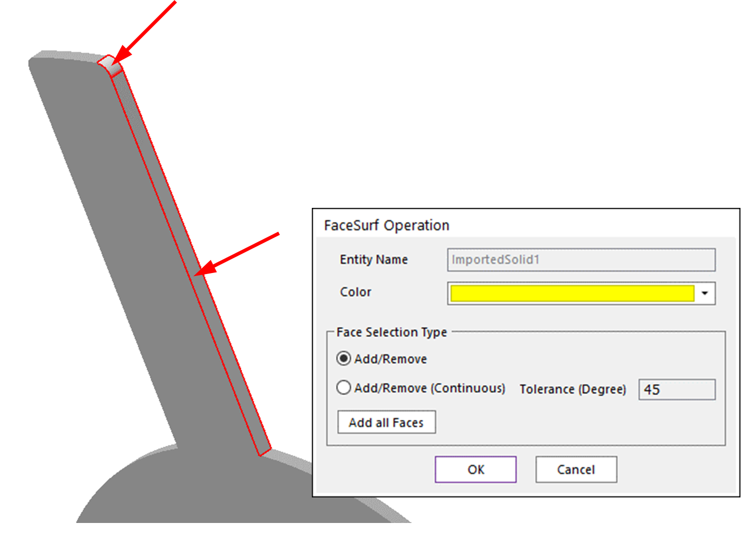
6. Change the color to Yellow.

7. Click OK.

7.1.4.5.2. To create the remaining face surfaces:

• Repeat the steps above, proceeding around the clutch driver, until all eight face surfaces have been created.

• Click Exit.

7.1.4.6. Creating the Contacts

Now that you have defined the necessary contact surfaces on the clutch plate and driver, you can create the contacts. (refer to the figure below shows the 12 regions where the contacts will be created)

7.1.4.6.1. Contact Layout Diagram

7.1.4.6.2. To create a driver arm contact:

In the 1 region, you can create a contact.

1. From the Contact group in the Professional tab, click the Geo Surface Contact function.

2. Set the Creation Method to Surface(PatchSet), Surface(PatchSet).

3. Select the first face surface that you had created on the clutch driver, as shown at below.

4. Select the first patch set that you had created on the FFlexClutchPlate, as shown at below.

   

7.1.4.6.3. To create the remaining driver arm contacts:

Repeat the steps above for the remaining driver-to-plate contacts (2-8 regions), proceeding clockwise around the clutch driver.

7.1.4.6.4. To create a plate-to-load contact:

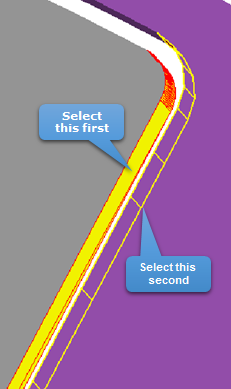
1. Repeat the same steps for creating a contact (9 region), but this time for the uppermost plate-to-load contact. Select the inner cylindrical surface of the load, as shown below. The edges of this surface are highlighted in light red when selecting it.

   

2. Select the uppermost patch set. As with the other patch sets.

7.1.4.6.5. To create the remaining plate-to-load contacts:

• Repeat the steps above for the remaining the plate-to-load contacts (10-12 regions), proceeding clockwise around the clutch driver.

• The model appears as shown next.

The icons for the contact clutter the display of the model and make upcoming steps more difficult. Because of this, you will turn off the display of the contacts, as well as the revolute joints and rotational axial forces.

7.1.4.6.6. To clean up the display of the model:

1. From Render Toolbar, click the Icon Control tool.

2. Clear the selection of the check boxes.

   

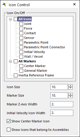
3. Close the Icon Control dialog box (use the x in the upper right corner).

7.1.4.7. Tuning the Contacts

Now that the contacts have been created, you will tune them. You will make certain changes to all the contacts, first, and then add friction to the plate-to-load contacts.

The friction characteristics of the plate-to-load contacts are important because the clutch relies on this friction to transfer power from the driver to the load. To keep the simulation time short, you will use a friction coefficient that is higher than the normal range.

For the driver arm contacts, you are less concerned with the friction. For these contacts, you will neglect friction to shorten the simulation time.

7.1.4.7.1. To tune the contacts:

1. In the Database Window, use the Shift key again to select all twelve contacts at once (GeoSurContact1 - GeoSurContact12).

2. Right-click the selected contacts and click Properties.

3. Click the Characteristic page.

4. Make the following changes:

   • Stiffness Coefficient: 50000

   • Damping Coefficient: 2.5

     

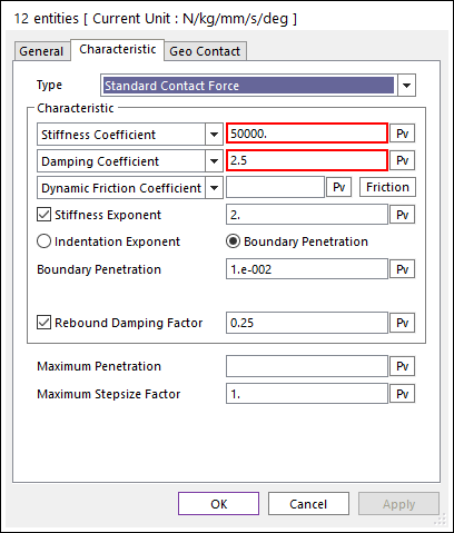
5. Click OK.

7.1.4.7.2. To add friction to the plate-to-load contacts:

1. In the Database Window, use the Shift key again to select the last four contacts (GeoSurContact9 - GeoSurContact12).

2. Right-click the selected contacts and click Properties.

3. Select the Characteristic page.

4. Make the following change:

   • Dynamic Friction Coefficient: 1.2

     

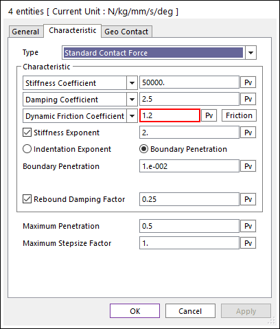
5. Click Friction.

6. Make the following changes:

   • Static Threshold Velocity: 10

   • Dynamic Threshold Velocity: 15

   • Static Friction Coefficient: 1.26

     

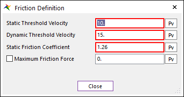
7. Click Close.

8. Click OK.

7.1.4.7.3. Save the model

7.1.5. Creating a Boundary Condition

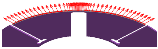
In this chapter, you will create a boundary condition for all the finite element nodes of the clutch plate. The boundary condition will limit the motion of these nodes in the Z-direction to zero. This will simulate the actual clutch, in which a structure would be in place to prevent the clutch plate from falling out of the clutch. In addition, it will reduce simulation time by reducing a degree of freedom for all elements.

7.1.5.1. Task Objective

Learn to set up a boundary condition for all the elements in the clutch plate.

7.1.5.2. Estimated Time to Complete

5 minutes

7.1.5.3. Creating a Boundary Condition

7.1.5.3.1. To set up a boundary condition:

1. In the Database Window, right-click FFlexClutchPlate, and click Edit.

2. From the FFlex Edit group in the FFlex Edit tab, click the Boundary Condition function.

3. Clear the check boxes next to the axes of motion, except for Z, as shown on the below.

   

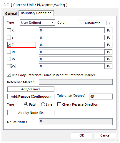
4. Click Add/Remove.

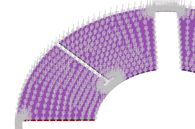
5. In the Working window, select all the nodes by clicking and dragging a select box around the entire clutch plate.

6. In the Working window, right-click, and click Finish Operation.

7. Click OK.

   The clutch plate now appears as shown below, with arrows pointing in the negative Z-direction.

   

8. Click Exit.

7.1.5.3.2. Save the model

7.1.6. Simulating the Model

In this chapter, you will run a simulation, enable contoured viewing of internal stresses, and play the simulation.

7.1.6.1. Task Objective

You will learn to:

• Set up and run a simulation.

• Enable the viewing of internal stresses.

• Plot and interpret the simulation results.

7.1.6.2. Estimated Time to Complete

15 minutes

7.1.6.3. Setting up and Running the Simulation

7.1.6.3.1. To set up and run the simulation:

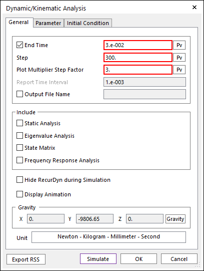
1. From the Simulation Type group in the Analysis tab, click the Dynamic/Kinematic Analysis function.

2. On the General page, make the following changes:

   • End Time: 3.e-02

   • Step: 300

   • Plot Multiplier Step Factor: 3

     

3. On the Parameter page, make the following change:

   • Initial Time Step: 1.e-06

   • Numerical Damping: 0.3

     

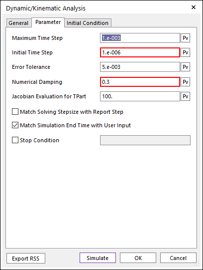
4. Click Simulate.

The simulation runs for 1 to 5 minutes.

7.1.6.4. Enabling Contoured View of Stresses in the Clutch Plate

To visualize the internal stresses in the clutch plate, enable the contour display.

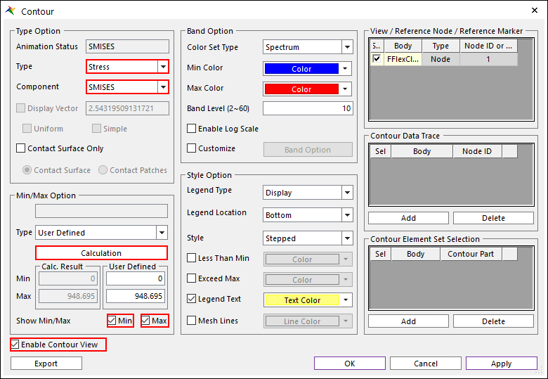
7.1.6.4.1. To enable the contour display:

1. From the FFlex group in the Flexible tab, click the Contour function.

2. Near the bottom of the dialog box, as shown in the figure on the below, select Enable Contour View.

3. In the Contour Option section, set Type to Stress.

4. At the bottom of the list, click SMISES.

5. Click Calculation.

   This determines the minimum and maximum stress that occurs throughout the simulation.

6. Click the checkbox next to Min and Max.

7. Click OK.

   Now that you have run the simulation and enabled contour display, you can play the animation.

   

7.1.6.5. Viewing the Animation Results

7.1.6.5.1. To play the animation:

• From the Animation Control group in the Analysis tab, click Play/Pause.

The animation shows the driver begin to spin and then contact the plate. As the plate and driver increase in rotational speed, the plate expands outwards and makes contact with the load. At the end of 0.03 second, the load rotates with the plate, but not at the same speed.

7.1.6.5.2. When the animation finishes:

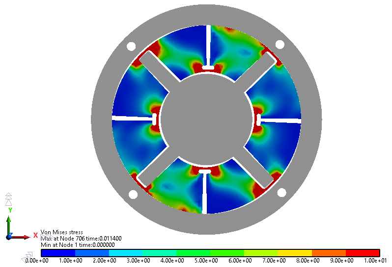
1. Examine where the areas of highest stress are. As expected, they are at the flex points.

   RecurDyn should also indicate which of the flex points has the highest stress.

2. Zoom into this part of the clutch plate, and view in Shade mode. It should appear as shown below.

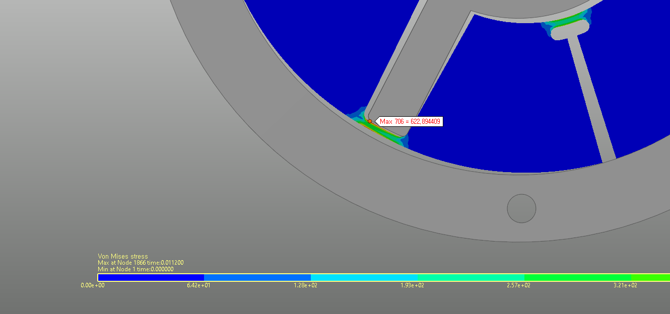
RecurDyn reports the node number and stress at the maximum stress point. At the middle of the simulation, the maximum stress is 622.89 N/mm2, occurring at Node 706.

Did you notice anything else about the results that you might not have expected? Even though the structure of the clutch is symmetrical, the deformation of the plate at the end of the simulation is asymmetrical. To examine why this occurred, adjust the scale and appearance of the contour plot as follows.

7.1.6.5.3. To adjust the contour display:

1. From the FFlex group in the Flexible tab, click the Contour function.

2. Under Min/Max Option, change Type to User Defined.

3. Set the Max to 10.

4. Clear Min and Max options.

5. Under Style Option, set Style to Smooth.

6. Check Exceed Max option.

7. Change Exceed Max Color to red

   

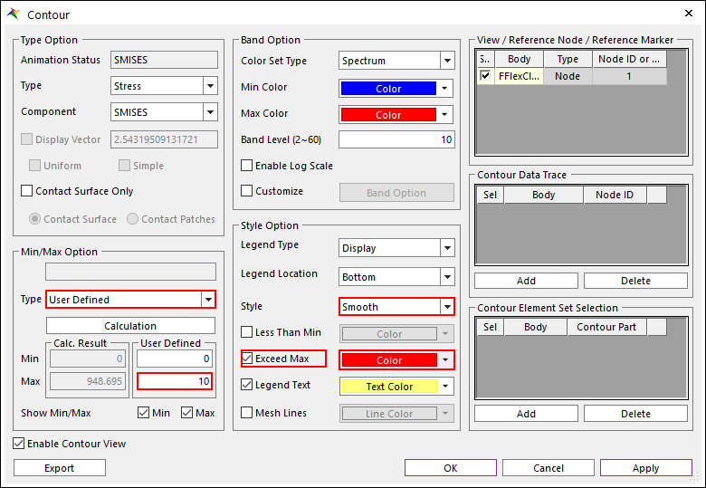
8. Click OK.

9. Play the animation again and observe the results.

With the given friction settings, this particular design shows instability, with a tendency to shift to an asymmetrical mode.

At some point during the animation, you see the results shown next.

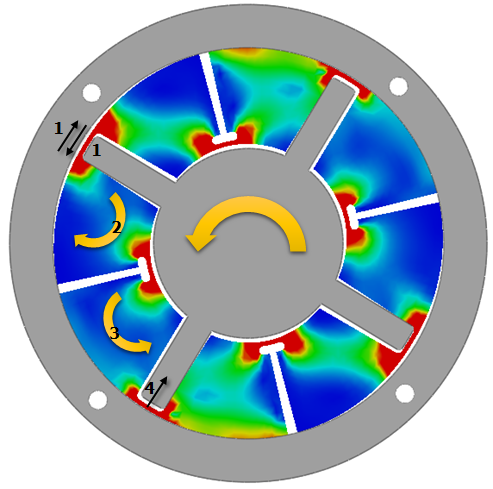
One explanation for the asymmetrical behavior could be as follows.

Forces (1) on the left plate segment from the clutch driver and load friction cause a clockwise torque (2) on the plate segment. The torque is transferred to the adjacent segment below, where it becomes a counterclockwise torque (3). The torque in turn pulls (4) the lower-left flex points away from the load, therefore, creating the asymmetry. The same chain of events occurs on the opposite side of the plate, as well.

You can confirm then from looking at the contour plots that the load path described above follows the areas of highest stress and ends where the stress begins to fade.

7.1.6.6. Plotting the Simulation Results

You will now use RecurDyn’s plotting capability to visualize more results. We assume that you have a basic knowledge of how to plot data in RecurDyn. If you need to review these methods, refer to the 3D Crank-Slider tutorial.

First, you will compare plots of rotational velocities and torques to the animation, in real time.

7.1.6.6.1. To compare rotational velocity and torque plots to the animation:

1. From the Plot group in the Analysis tab, click the Plot Result function.

2. From the Windows group in the Home tab, click the Show All Windows function.

3. In the upper left window, click the Load Animation function from the Animation group in the Tool tab.

4. In the upper right window, plot the rotational velocities of the clutch driver and load:

   • FFlexClutch -> Bodies -> ClutchDriver -> Vel_RZ

   • FFlexClutch -> Bodies -> ClutchLoad -> Vel_RZ

5. In the lower right window, plot the torques applied to the clutch driver and load:

   • FFlexClutch -> Force -> Rotational Single (Axial) Force -> RotAx_driver -> TZ_Rotat_Axial

   • FFlexClutch -> Force -> Rotational Single (Axial) Force -> RotAx_load -> TZ_Rotat_Axial

   Your Plot windows appear as shown below.

   

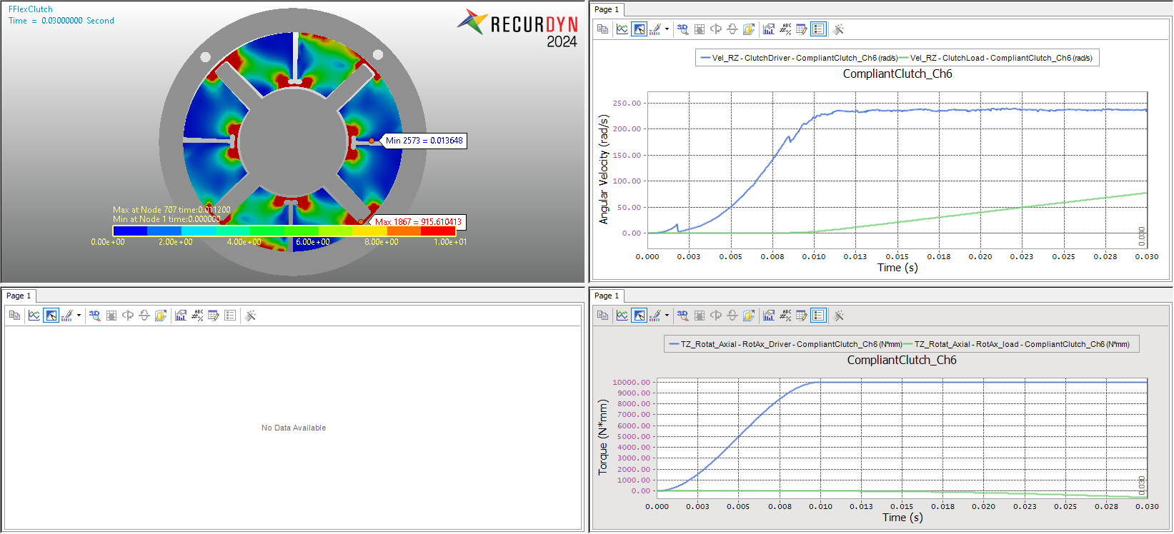
6. Play the animation.

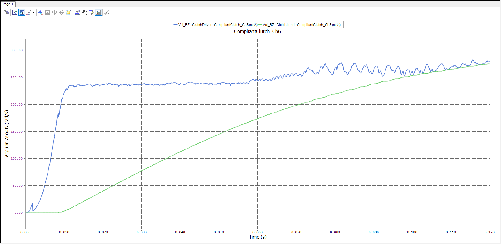
Looking at the plot below, it is apparent that the two velocities will probably converge sometime in the future. What significant events occur at points 1 and 2?

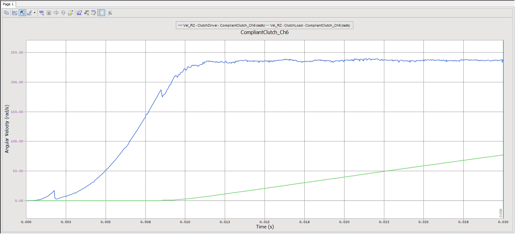
Answers: (1) The clutch driver makes contact with the clutch plate, which initially starts in a floating position, and (2) the clutch plate assumes an asymmetric shape.

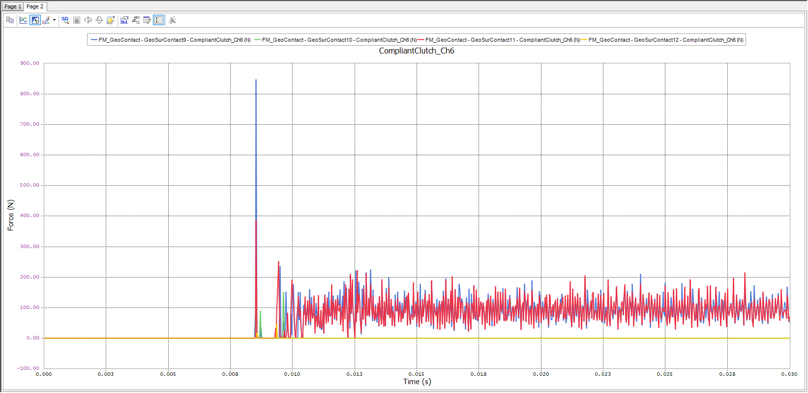
You will now plot the contact forces experienced by the driver arm and plate-to-load contacts. Recall that contacts 1 through 8 are the driver arm contacts, and contacts 9 through 12 are the plate-to-load contacts.

7.1.6.6.2. To plot the contact forces:

1. In a new Plot window, plot the four driver arm contact forces that experience contact during the simulation.

   These will be for contacts 2, 4, 6, and 8 (FFlexClutch -> Contact -> GeoContact -> GeoSurContact2 -> FM_GeoContact , and so on).

2. In another Plot window, plot the four-clutch plate-to-load contact forces.

   These will be for contacts 9 through 12 (FFlexClutch -> Contact -> GeoContact -> GeoSurContact9 -> FM_GeoContact , and so on).

Your plots appear as shown next.

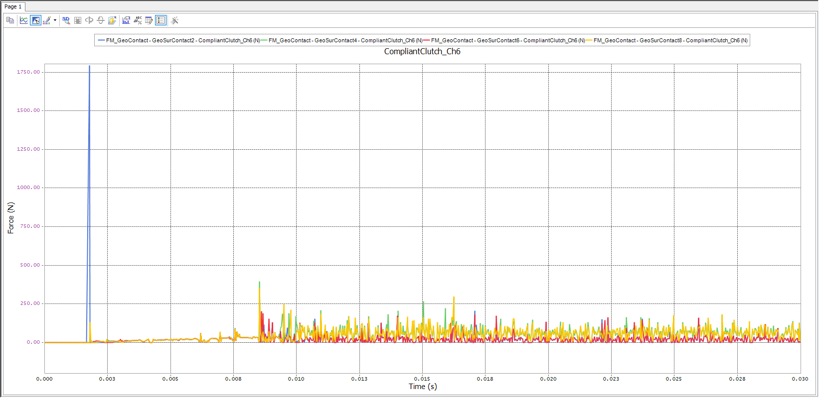
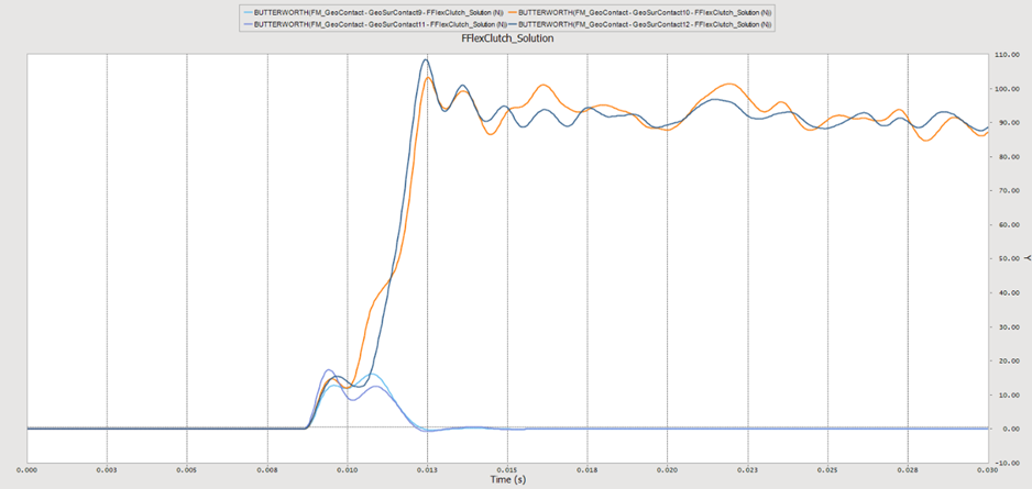
These plots are interesting but can be made easier to interpret by reducing the noise in the data. You will now apply a low-pass filter to the data, using a cut-off frequency of 600 Hz.

Note

The FM_CONTACT_BASE plot option takes the value of the total force experienced by the contact. This is why the units in the plots above are force, not force/area.

7.1.6.6.3. To apply a filter to the contact force data:

1. Click the Filter function of the Analysis group in the Tool tab.

2. Use the figure below for the next several steps.

3. Change the Type to Low Pass (click on the field to enable the dropdown button and make the selection from the dropdown list).

4. Set Cutoff (Hz) to 600.

5. Click Execute.

6. Set Curve to 1: FM_GeoContact – GeoSurContact2 (N), again by activating the dropdown list in the field.

7. Click Execute.

8. Repeat the two steps above for the three remaining curves of interest.

9. Click Close.

   When finished applying the filters, note that the filter causes a small-time lag.

10. To clean up the plot, delete the unfiltered plot lines and change the new plot colors as desired to make each line more distinct.

11. Repeat the steps above for the other contact force plot.

Your plots should now appear as shown next.

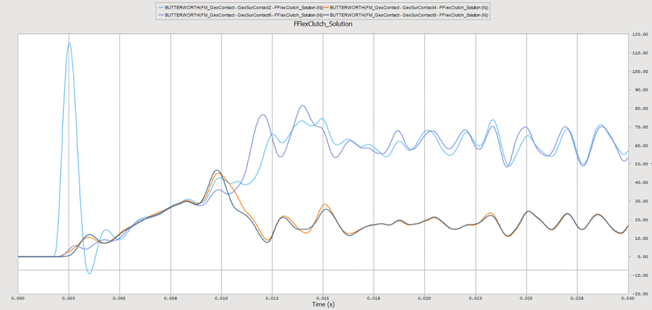
The plots are now much easier to interpret. Looking at the driver arm contacts; all four contacts experience similar forces until contact is made between the plate and load. At this point, contacts 2 and 6 oscillate opposite contacts 4 and 8, with contact 4 and 8 ultimately maintaining higher contact forces. This makes sense because contacts 4 and 8 are on the driver arms whose surrounding plate segments are those that end up making more contact with the load, and, therefore, transfer more of the torque. Interestingly, the divergence of contacts 2/6 from 4/8 occurs at ~0.010 sec., some time before the clutch plate assumes an asymmetrical shape (~0.016 sec.).

Looking at the clutch plate-to-load contacts, contacts 9 and 11 are similar, and 10 and 12 are similar. The 9/11 group and the 10/12 group initially oscillate in the same direction, but as time progresses, the oscillation becomes opposite, and the 9/11 group assumes the higher contact forces. These contacts are on the top and bottom of the clutch plate in its starting position and are the ones that end up having more contact with the load.

Finally, you might wonder how long it takes the clutch to engage. If you were to run the simulation longer, you would obtain the results below, which show that the clutch engages at 0.095 seconds.

7.1.7. Appendix A: Creating the Remaining Patch Sets

This appendix continues the section, Creating the Patch Sets, explaining how to create the remaining eight patch sets required for the surface contacts. It provides you with more experience creating patch sets.

7.1.7.1. Task Objective

You will practice creating patch sets.

7.1.7.2. Estimated Time to Complete

25 minutes

7.1.7.3. Creating the Remaining Patch Sets

7.1.7.3.1. To create the remaining patch sets:

1. Using the same method (Add/Remove(Continuous) ) used to create the first patch set, select the surfaces the clutch plate as indicated in the contact layout diagram at the beginning of this appendix.

   As you proceed, RecurDyn automatically names the patch sets SetPatch2, SetPatch3, …, SetPatch8.

2. Repeat the same steps for the outer surfaces of the clutch plate, starting with the upper surface and going clockwise around the clutch plate, as indicated in the contact layout diagram. For each surface, select the elements as shown below, highlighted in light gray:

   

   The normals should all point outwards towards the clutch load, as shown below:

   

3. Click the Exit function to return to the root model.

4. Continue with the section, Creating the Face Surfaces.