9.6. Media Transport System Tutorial (MTT2D)

9.6.1. Getting Started

9.6.1.1. Objective

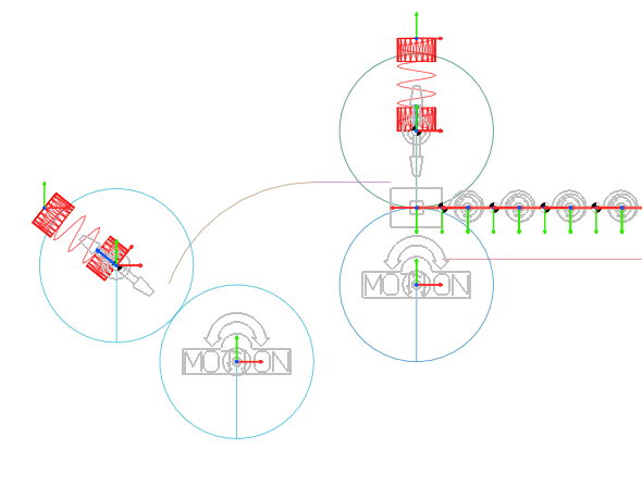
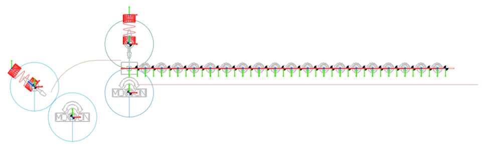
This tutorial acquaints you with the basic operation of the 2D Media Transport Toolkit (MTT2D). You will learn how to create and use a sheet group to represent the media (paper or film), fixed and moveable rollers to drive the media, and linear and arc guides to guide the motion of the media. In this tutorial, you will create the media transport model shown below:

The tutorial consists of two chapters demonstrating the basics of the MTT2D, followed by three optional exercises. Each optional exercise is independent of the other optional exercises. You can choose to work with any of the optional exercises after creating the model as instructed in Chapters 2 and 3. You do not have to run the simulation or plot the results before moving on to the optional exercises.

9.6.1.2. Audience

This tutorial is intended for experienced users of RecurDyn. All new tasks are explained carefully.

9.6.1.3. Prerequisites

Users should first work through the 3D Crank-Slider, Engine with Propeller, and Pinball (2D contact) tutorials, or the equivalent. We assume that you have a basic knowledge of physics.

9.6.1.4. Procedures

The tutorial is comprised of the following procedures. The estimated time to complete each procedure is shown in the table.

Procedures	Time (minutes)
Simulation environment set up	5
Media transport model creation and analysis	30
Optional exercise 1	15
Optional exercise 2	15
Optional exercise 3	15
Total	80

9.6.1.5. Estimated Time to Complete

This tutorial takes approximately 80 minutes to complete.

9.6.2. Setting Up Your Simulation Environment

In this chapter, you will create a new media transport subsystem and set up the simulation environment.

9.6.2.1. Task Objective

Learn how to create a new media transport subsystem.

9.6.2.2. Estimated Time to Complete

5 minutes

9.6.2.3. Starting RecurDyn

9.6.2.3.1. To start RecurDyn and create a new model:

1. On your Desktop, double-click the RecurDyn icon. RecurDyn starts and the Start RecurDyn dialog appears.

2. Enter the name of the new model as MTT2D_Example.

3. Click OK.

9.6.2.4. Creating a New Media Transport Subsystem

All the tools to create and work with a MTT2D model are in the MTT2D toolkit under the Subsystem tab in the Toolkit bar.

9.6.2.4.1. To create a MTT2D model:

1. From the Subsystem Toolkit group in the Toolkit tab, click the MTT2D function.

2. RecurDyn is now in subsystem edit mode.

9.6.2.5. Setting Up the RecurDyn User Environment

Now, set up the RecurDyn environment so it is easier to work with the MTT2D model.

9.6.2.5.1. To set up the RecurDyn environment:

1. Set the grid size to 5.

   

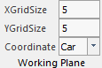
2. Set the icon and marker size to 5.

3. Use the Zoom tool or type z and drag up or down until the grid of points just fits in the screen.

9.6.3. Creating and Analyzing the Media Transport Model

In this chapter, you will create the media transport model and investigate the loads on the:

• Mean sheet slip to moveable rollers

• Sheet segments

9.6.3.1. Task Objective

Learn to:

• Create the sheet

• Create the rollers and linear guides

• Define roller motion

• Run simulations and plot results

9.6.3.2. Estimated Time to Complete

30 minutes

9.6.3.3. Creating the Sheet

You will begin by creating the sheet.

9.6.3.3.1. To create the sheet:

1. Form the Sheet group in the MTT2D tab, click the Sheet function.

2. Set the Creation Method to Point, Point, Withdialog:

   • Sheet Start Point: -10, 120, 0

   • Sheet End Point: 30, 120, 0

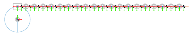
3. Review the Sheet dialog box and make changes as needed (typically no changes are needed) to match the figure on the below and listed below and click OK:

   • Sheet Start Point: -10,120,0

   • Sheet Direction Point: 30, 120, 0

   • Number of Sheet Segment: 20

   • Segment Length: 10

   • Sheet Thickness: SH_T 0.5

   • Density: SH_D 2.2e-06

   • Young’s Modulus: SH_E 2250

   • Damping Factor: SH_C 32

   • Sheet Curl Radius: SH_CR 0

     

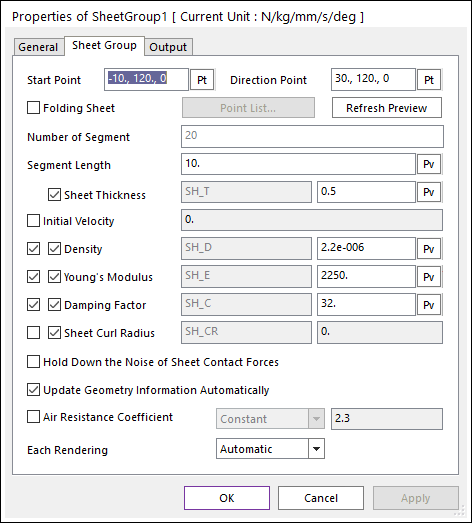
4. Folding Sheet, Initial Velocity, Air Resistance Coefficient, and Hold Down the Noise of Sheet Contact Forces are not selected.

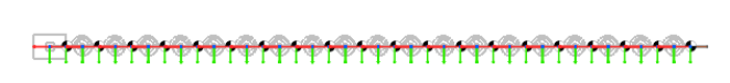
5. The sheet appears in the graphics window as shown below.

   

6. Save the file to a working directory as MTT2D_Example.rdyn.

9.6.3.4. Creating Roller Pair 1

Roller pair 1 consists of the following rollers, which you will create in the next steps:

• Fixed

• Movable

9.6.3.4.1. To create a fixed roller:

1. From the Roller group in the MTT2D tab, click the Fixed Roller function.

2. Set the Creation Method to Point, Radius:

   • Roller Center Point: -10, 105, 0

   • Roller Radius Point: 15 (or enter 15 in the Input Window toolbar)

Your model looks like the following:

9.6.3.4.2. To create the movable roller:

1. From the Roller group in the MTT2D tab, click the Movable Roller function.

2. Set the Creation Method to FixedRollerGroup, Direction, Radius.

3. Click the Fixed Roller Group that you just created, and the two points shown below:

   • FixedRollerGroup: FixedRollerGroup1

   • Roller Direction Point: 0, 1, 0

   • Roller Radius Point: 15 (or enter 15 in the Input Window toolbar)

   The fixed roller and sheet appear in the modeling window as shown below.

   

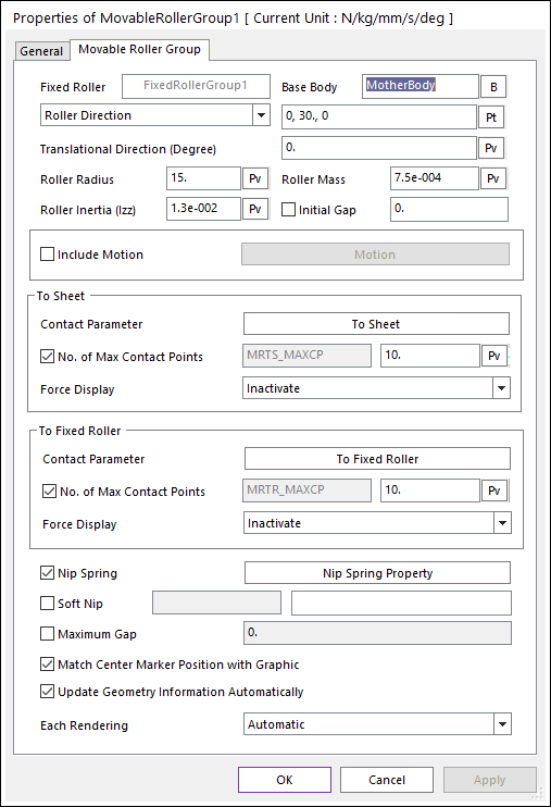
4. If you would like to, you can look at the properties of the Movable Roller, which should match the dialog box shown on the below and listed below.

   Tip

   Right-click the Movable Roller Group1 and click Properties.

   • Base Body: MotherBody

   • Roller Direction: 0, 1, 0

   • Roller Radius: 15

   • Roller Mass: 7.5e-04

   • Roller Inertia (1zz): 1.3e-02

   Nip Spring, Match Center Marker Position with Graphic, and Update Geometry Information Automatically are all selected.

   

9.6.3.5. Creating Roller Pair 2

In this section, you will use the Roller Pair tool, which creates both a fixed and a moveable roller in a single operation.To create the roller pair:

9.6.3.5.1. To create the roller pair:

1. From the Roller group in the MTT2D tab, click the Pair Roller function.

2. Set the Creation Method to Point, Radius, Direction, Radius:

   • Center Point: -45, 90, 0

   • Radius Point: 15 (or enter 15 in the Input Window toolbar)

   • Direction: -0.781, 0.625, 0

     Tip

     Use the coordinate readout at the bottom right area of the RecurDyn window (Global X:-70 Y:110 Z:0) to determine the cursor location.

   • Radius Point: 15 (or enter 15 in the Input Window toolbar)

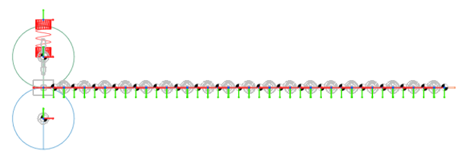
   The model now looks like the one shown on the below.

   

3. Again, save the file to a working directory.

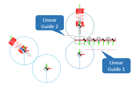
9.6.3.6. Creating Two Linear Guides

Now, you will create two linear guides: one defined from left to right and one from right to left.

9.6.3.6.1. To create the linear guides:

1. Before you begin, to get a better view of the model, fit it to the screen and zoom out approximately 10%.

2. From the Guide group in the MTT2D tab, click the Linear Guide function.

3. Set the Creation Method to Point, Point.

4. Click each pair of points as shown below. Note that each guide pushes against the sheet in one normal direction. The convention is that a horizontal guide that is defined from left to right pushes in the upward direction.

   • Linear guide 1:

     • Start Point: -5, 110, 0

     • End Point: 205, 110, 0

     Note

     Guide defined from left to right; contacts sheet in the upward direction.

   • Linear guide 2:

     • Start Point: -15, 125, 0

     • End Point: -30, 125, 0

     Note

     Guide defined from right to left; contacts sheet in the downward direction.

The model appears as shown below.

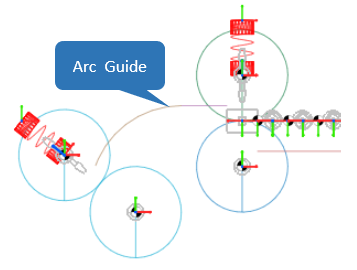
9.6.3.7. Creating an Arc Guide

9.6.3.7.1. To create an arc guide

1. From the Guide group in the MTT2D tab, click the Arc Guide function.

2. Select the Creation Method to Point, Point, Direction, Angle:

   • Center Point: -30, 95, 0

   • Radius Point: -30, 125, 0

   • Direction Point: -1, 0, 0 (or any point to the left of the radius point)

   • Angle Point: -60, 105, 0 (or enter 70 into the Input Window toolbar)

     Tip

     Use the coordinate readout at the bottom right area of the RecurDyn window (Global X:-60 Y:105 Z:0) to determine the cursor location.

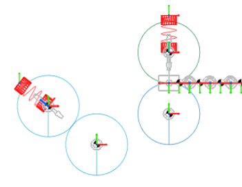
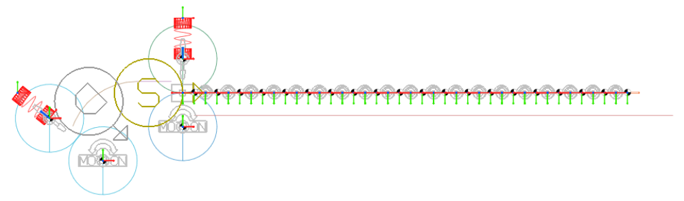
   • The model now appears as shown on the below.

     

3. Again, save the file to a working directory.

9.6.3.8. Defining Roller Motion

In this section, you set the input motion of the two fixed rollers by adding a motion input to each fixed roller group. The motion will be applied to each revolute joint as shown in the figure on the below.

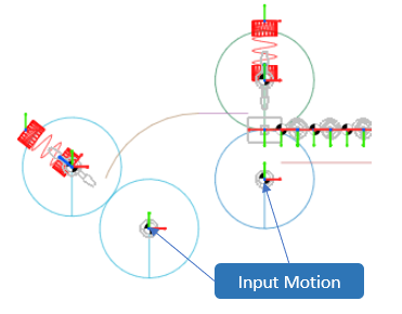
9.6.3.8.1. To define the roller motion:

1. Open the Properties dialog box for the first fixed roller group, FixedRollerGroup1.

2. Check the Include Motion option.

3. Click Motion.

4. Click EL to view the expression list.

5. Click Create.

6. Type the motion expression into the Expression area as shown in the dialog box on the below:

   • 2*TIME

     

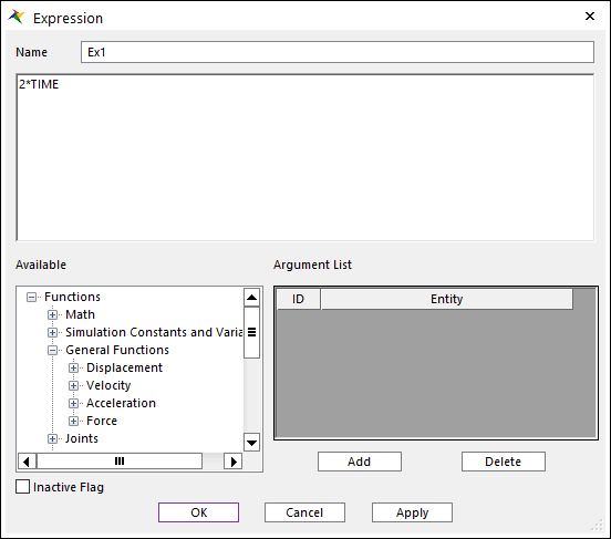
7. Click OK on each of the four dialog boxes to complete the definition.

8. Repeat the process with the second fixed roller group, FixedRollerGroup2, except that you can simply reuse the same motion expression that you created in the earlier step by selecting the expression from the Expression List.

When you have completed these steps, the model appears as shown below.

9.6.3.9. Running the Dynamic Simulation

9.6.3.9.1. To run the dynamic simulation:

1. From the Simulation Type group in the Analysis tab, click the Dynamic /Kinematic Analysis function.

2. In the Dynamic Analysis dialog box, set the following:

   • End time: 5

   • Number of steps: 100

   • Plot Multiplier Step Factor: 5

   • Check Hide RecurDyn during Simulation.

3. Click Simulate.

4. Check the status of the simulation by placing the cursor over the RecurDyn icon in the task bar at the bottom of the screen.

5. The simulation completes in less than a minute.

6. From the Animation Controls group in the Analysis tab, click the Play function.

9.6.3.10. Plotting Results

9.6.3.10.1. To plot the output data:

1. From the Plot group in the Analysis tab, click the Plot Result function.

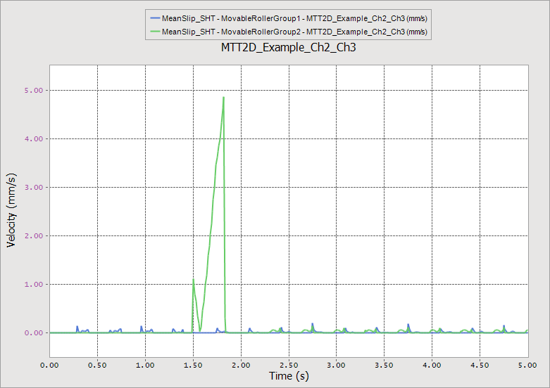
2. In the Plot Database Window on the right, expand Movable Roller -> MovableRollerGroup1 and MovableRollerGroup2.

   Double-click MeanSlip_SHT in each section and adjust the labels and axes to obtain the plot below. You can see large amount of registered slip when the leading edge of the sheet stubs up against the movable roller of the second roller pair.
   

3. From the Windows group in the Home tab, click the Add Page function.

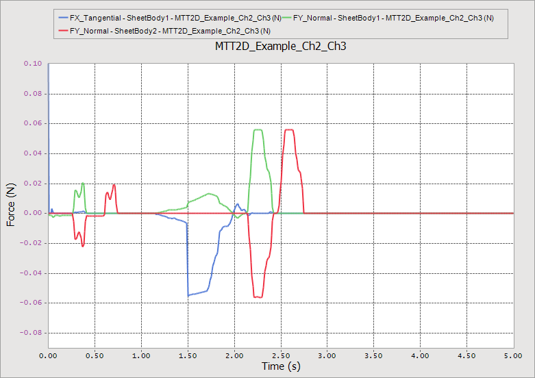
4. In the Plot Database Window, expand SheetBody -> SheetBody1.

5. Double-click FX_Tangential and FY_Normal.

6. Expand SheetBody2 and double-click FY_Normal.

7. Adjust the labels and axes to obtain the plot shown next.

   

8. Close the plot window.

9. RecurDyn returns to the modeling window.

10. Save your RecurDyn model file.

You can stop with this tutorial now or you can work through the following optional exercises. Each optional exercise is independent of the other optional exercises.

9.6.4. Optional Exercise 1 - Adding Speed and Distance Sensors

9.6.4.1. Task Objective

In this exercise, you will define two sensors:

• Speed sensor to measure the velocity of the sheet in the x direction

• Distance sensor to measure the closest distance between the sheet and a certain point on the arc guide

You will then run a simulation and plot the sensor results.

9.6.4.2. Estimated Time to Complete

15 minutes

9.6.4.3. Setting Up the Model

You will open the model you created in the previous exercise and save it as a new name.

9.6.4.3.1. To set up the model:

1. Open the file MTT2D_Example.rdyn that you created by performing the major steps in the first two chapters of this tutorial.

2. From the File menu, choose the Save As function and save a new model file as MTT2D_Example_Sensor.rdyn.

9.6.4.4. Creating the Speed Sensor

Next, you will use a speed sensor to measure the velocity of the sheet in the x direction.

9.6.4.4.1. To create the speed sensor:

1. From the Sensor group in the MTT2D tab, click the Speed Sensor function.

2. Set the Creation Method to Point, Direction, Distance.

3. And enter the following:

   • Center Point: -25, 120, 0

   • Direction Point (+X): 1, 0, 0 (or enter 1,0,0 in the Input Window Toolbar)

   • Distance Point: 15 (or enter 15 in the Input Window Toolbar)

9.6.4.5. Creating a Distance Sensor

You will use a distance sensor to measure the closest distance between the sheet and a selected point on the arc guide.

9.6.4.5.1. To create a distance sensor:

1. From the Sensor group in the MTT2D tab, click the Distance Sensor function.

2. Set the Creation Method to Point, Direction, Distance.

3. And enter the following:

   • Center Point: -51.2, 116.2, 0 (along arc, 45 degrees from vertical)

   • Direction Point: Enter 1, -1, 0 in the Input Window Toolbar to define a direction of 45 degrees, which is normal to the arc at the center of the distance sensor.

   • Distance Point: Enter 15 in the Input Window Toolbar.

When you complete these steps, the model should appear as shown below.

9.6.4.6. Running the Dynamic Simulation

9.6.4.6.1. To run the dynamic simulation:

1. From the Simulation Type group in the Analysis tab, click the Dynamic / Kinematic Analysis function.

2. Set the following:

   • End time: 5

   • Number of Steps: 100

   • Plot Multiplier Step Factor: 5

   • Check Hide RecurDyn during Simulation

3. Click Simulate.

4. Check the status of the simulation by placing the cursor over the RecurDyn icon in the task bar at the bottom of the screen.

5. The simulation completes in less than a minute.

6. Press the Play function of the Animation Control group in the Analysis tab to play the animation and verify that the addition of the sensors did not affect the behavior of the model.

9.6.4.7. Plotting the Results

9.6.4.7.1. To plot the sensor output data:

1. From the Plot group in the Analysis tab, click the Plot Result function.

2. In the Plot Database Window on the right, expand Sensor -> SpeedSensor1.

3. Double-click Value to draw the curve of sheet velocity.

   

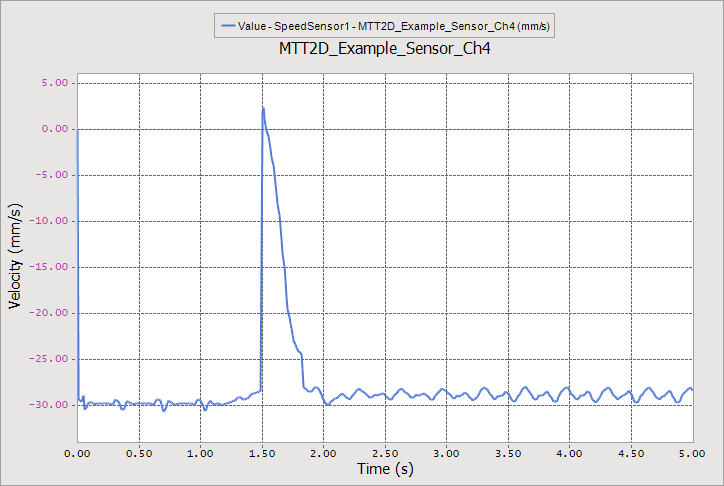
   Note that the sheet comes to a halt and reverses slightly between 1.5 and 1.85 seconds. A review of the animation shows that interaction between the leading edge of the sheet and the second movable roller causes this behavior.

4. From the Windows group in the Home tab, click the Add Page function. (Create a new plot page.)

5. In the Plot Database Window, expand DistanceSensor1.

6. Double-click Value to draw the distance curve.

7. Adjust the labels and axes to obtain the plot shown below.

   

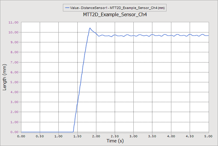
   Note that the distance of the sheet from the arc guide is greatly influenced by its entry into the second roller pair.

8. Close the plot window.

9. Save your RecurDyn model file.

9.6.5. Optional Exercise 2 – Reverse Sheet Direction

9.6.5.1. Task Objective

In this exercise, you will use an event sensor to measure when the sheet has entered into the second roller pair. The roller motion will be reversed 0.5 seconds after the sensor detects the sheet entrance.

9.6.5.2. Estimated Time to Complete

15 minutes

9.6.5.3. Setting Up the Model

9.6.5.3.1. To set up the model:

1. Open the file MTT2D_Example.rdyn that resulted from performing the steps in the main section of the tutorial.

2. From the File menu, choose Save As and to save the new model file as MTT2D_Example_Rev.rdyn.

3. Click the right mouse button over the subsystem MTT2D1 and select the Edit option to enter the subsystem mode for this subsystem that you created in the first section of the tutorial.

9.6.5.4. Creating an Event Sensor

In this section, you will create an event sensor. An event sensor provides two pieces of information:

• The SNSR function expression has a value of 0 before the event occurs and a value of 1 after the event occurs.

• The EVTIME function expression holds the simulation time when the event occurs.

You will use the STEP function to blend in the change of roller velocity at 0.5 seconds after the event occurs. You will modify the Input Motion Expression of the two fixed rollers to use the information from the event sensor.

9.6.5.4.1. To create an event sensor:

1. From the Sensor group in the MTT2D tab, click the Event Sensor function.

2. Set the Creation Method to Point, Distance:

   • Center Point: Enter -57, 100, 0 in the Input Window Toolbar.

   • Distance: Enter 5 in the Input Window Toolbar.

3. In the Database window, right-click the expression Ex1, and click Properties.

4. Click E on the row with expression Ex1 in the Expression list and modify the motion expression as follows:

   • 2*TIME - SNSR(1)*STEP(TIME, EVTIME(1)+0.5, 0, EVTIME(1)+0.6, 2)*2*(TIME-EVTIME(1)-0.5)

     

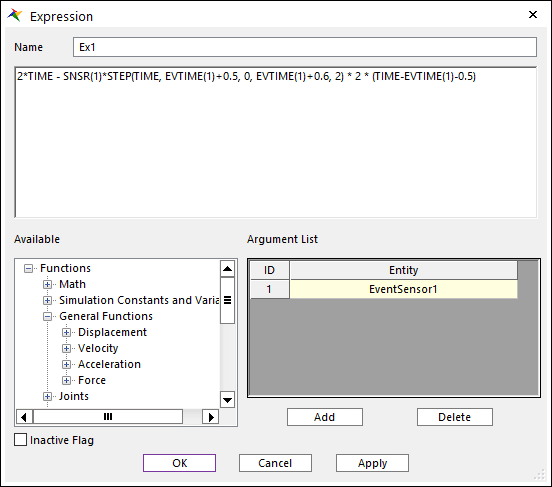
5. Click Add in the lower right corner of the Expression dialog box to add a text box to the Argument List.

6. From the Database Window, drag the EventSensor1 item in the Sensors group to the text box just created in the Argument List.

7. Click the Dynamic / Kinematic Analysis function and following the procedure given in the basic tutorial for running a simulation.

8. Press the Play function on the Animation Control group to play the animation and you will see the reversal of the roller motion 0.5 seconds after the sheet passes through the second roller pair.

9. Save your RecurDyn model file.

9.6.6. Optional Exercise 3 – Checking the Sensitivity of Model

9.6.6.1. Task Objective

In this exercise, you will modify the model you created in the main section of the tutorial to see its sensitivity.

9.6.6.2. Estimated Time to Complete

15 minutes

9.6.6.3. Setting Up the Model

9.6.6.3.1. To set up the model:

1. Open the file MTT2D_Example.rdyn that resulted from performing the steps in the main section of the tutorial.

2. From the File menu, choose Save As to save a new model file as MTT2D_Example_Delta.rdyn.

9.6.6.4. Modifying the Model

9.6.6.4.1. To modify the model:

• Make the following modifications and run a simulation after each modification. Notice the effect that each change has on the behavior of the model.

• Double the velocity of the fixed rollers and run the simulation for 2.5 seconds.

• Change the sheet thickness to 0.2 mm and run the simulation for 2.5 seconds.

• Change the sheet thickness to 0.1 mm and run the simulation for 2.5 seconds.

• Is the simulation time getting shorter or longer? Why?

• Do you notice any contact problems? Why are they happening?

• Increase the contact damping on the arc guide by 10 times (.012 to .12).