10.1. Water Sloshing (Particleworks)

10.1.1. Getting Started

In this tutorial, you will learn how to perform a simulation in which Particleworks is co-simulated with RecurDyn. Co-simulation of Particleworks with RecurDyn allows fluids to be co-simulated with a multibody dynamics system. RecurDyn is used to analyze the MBD (Multi Body Dynamics) system, and Particleworks is used to analyze a fluid. The fluid dynamics formulation that Particleworks is based on is the MPS (Moving Particle Simulation) method.

The model that is used in this tutorial is based on a model used in a scientific journal paper in which fluid sloshing behavior and pressure in a rectangular tank is analyzed. The issue of sloshing is one of the most studied phenomena of fluid motion. There has been extensive research performed in this area as intense sloshing flow could result in significant damage to a Wall and its structure from the impact caused by fluid. The paper that is used as the basis of this tutorial compares the result analyzed using the CIP (Constrained Interpolation Profile) method, one of the fluid dynamics modeling methods, to the result gained from experimental trials. This tutorial will demonstrate how to compare and analyze the result from the MPS method in Particleworks and the results from the paper.

Reference: Numerical simulation of violent sloshing by a CIP-based method, Kishev etal (2006)

10.1.1.1. Objective

In this tutorial, you will learn how to:

• Create a rigid body model in and export *.wall files from RecurDyn

• Create particles in Particleworks

• Set fluid properties in Particleworks

• Co-simulate Particleworks with RecurDyn

• Post-process in Particleworks

10.1.1.2. Prerequisites

• This tutorial is intended for users who are familiar with the basic RecurDyn tutorials. Prior knowledge of the aforementioned tutorials will help you better understand this tutorial.

• Particleworks have to be installed to proceed with this tutorial. And this tutorial is progressed with Particleworks 7.1.0 version.

• This tutorial is progressed with the graphic card (NVIDIA GeForce GTX TITAN Black). The computer specification or software version can change the result of simulation.

10.1.1.3. Procedures

The tutorial is comprised of the following procedures. The estimated time to complete each procedure is shown in the table.

Procedures	Time (minutes)
Register Particleworks GUI in RecurDyn	10
Model creation in RecurDyn	15
Model creation in Particleworks	15
Co-simulation	120
Particleworks Post-processing	30
Analysis and review	5
Total	195

10.1.2. Register Particleworks GUI in RecurDyn

By default, the External SPI (Particleworks) GUI is not visible in the RecurDyn. You must add the GUI to RecurDyn using the configuration XML file provided by Particleworks.

10.1.2.1. Task Objective

Learn how to register External SPI(Particleworks) tab in RecurDyn ribbon using the configuration XML and to set a particle solver DLL.

10.1.2.2. Estimated Time to Complete

10 minutes

10.1.2.3. Copy Configuration XML

10.1.2.3.1. To copy Particleworks.xml:

Copy the Particleworks.xml from install path of Particleworks software.

- <Particleworks Install Path>\share\recurdyn\Particleworks_V9R5.xml

10.1.2.3.2. To paste XML in RecurDyn:

Paste the Particleworks.xml copied above to RecurDyn install path.

- <RecurDyn Install Path>\Bin\Solver\CoSim\StdParticleInterface\Particleworks_V9R5.xml

10.1.2.3.3. To confirm RecurDyn GUI:

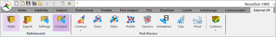
Run RecurDyn and check a ribbon GUI, you can see the External SPI tab and there is a Particleworks group.

10.1.2.3.4. To check a path of particle solver DLL:

Must check where particle solver DLL file should be located.

1. From the Particleworks group in the External SPI tab, click the Settings function.

2. In the Settings dialog box, click Info.

   

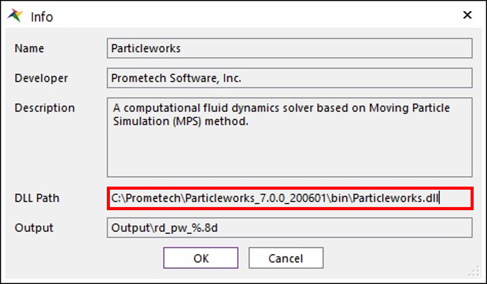
   You can check the DLL Path in the Info dialog window. This path is set to the default installation location of Particleworks. So if you installed Particleworks in a different path, you must modify the DLL path in the Configuration XML file.

   Tip

   Modifying the Particle Solver DLL path in Configuration XML file

   (Perform it when the DLL path in the Info dialog window is different from the Particleworks installation path.)

   1. Open the Particleworks.xml file.

   2. Modify the DLL path following <Path> as shown below.

      

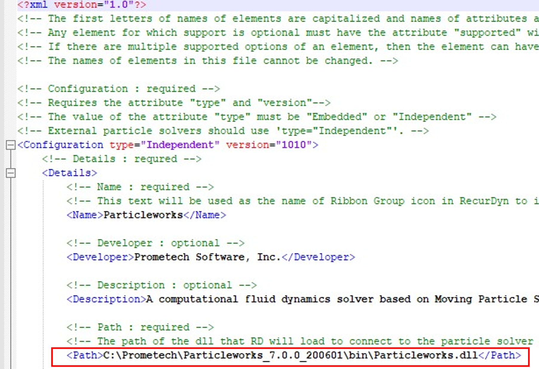
   3. Save the Configuration XML file.

   4. After confirming that the Configuration XML has been modified successfully, restart RecurDyn.

10.1.3. Creating a Model in RecurDyn

For co-simulation of Particleworks with RecurDyn, first, it is necessary to create a multibody dynamics model in RecurDyn. Then it is necessary to export certain data from that model that is required in Particleworks. In the second chapter, you will create a multibody dynamic model of the tank in which the fluid will slosh from side to side and then export the necessary files for Particleworks.

10.1.3.1. Task Objective

Learn how to create a multibody dynamic model necessary for analysis and how to export the necessary files for Particleworks.

10.1.3.2. Estimated Time to Complete

15 minutes

10.1.3.3. Starting RecurDyn

10.1.3.3.1. To start RecurDyn and create a new model:

1. On your Desktop, double-click the RecurDyn icon. RecurDyn starts and the Start RecurDyn dialog box appears.

2. Enter Sloshing for the Name of the new model.

3. Set Unit to MKS.

4. Click OK.

10.1.3.3.2. To save the model

• From the File menu, click Save As to save Sloshing.rdyn in the desired location.

  (In chapter 3, this model will be moved to the project folder in Particleworks.)

10.1.3.4. Creating the Geometry

Now, you will create the Container geometry.

1. Change the Working Plane to the XY Plane.

2. From the Body group in the Professional tab, click the Box function.

3. Set the Creation Method to Point, Point, Depth.

4. Enter the following in the Input Window Toolbar:

   • Point1: -0.3, 0, 0

   • Point2: 0.3, 0.3, 0

   • Depth: 0.05

5. Change the name of Body1 to Container.

6. Right-click on Container in the database window and then enter Edit Mode for the Container body.

7. From the Local group in the Geometry tab, click the Shell function.

8. Select Box1 on the Working Window.

9. Display the Shell Operation dialog box and do the following as shown in the figure to the below.

   • Value: 2.e-0.02

   • Direction: Outward

     

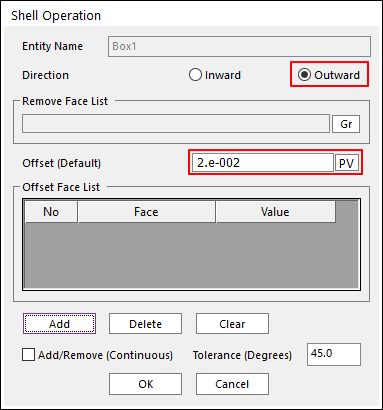
10. Click OK to exit the Shell Operation dialog box.

    

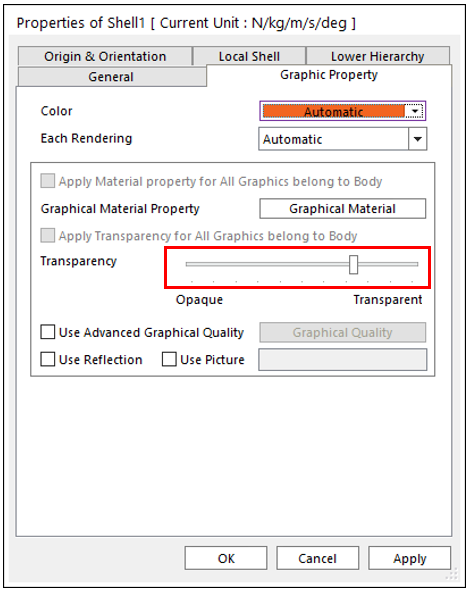
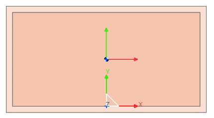
11. Raise the Transparency of Shell1 in the Graphic Property page in the Properties of Shell1 dialog box.

    You will see that the shell geometry of 0.02m in thickness has been created.

    

12. Exit Edit Mode.

10.1.3.5. Creating the Translational Joint

Now, you will create the joint to swing the Container body from side to side.

1. From the Joint group in the Professional tab, click the Translate Joint function.

2. Set the Creation Method to Body, Body, Point, Direction.

3. Enter the following in the Input Window Toolbar:

   • Body 1: Ground

   • Body 2: Container

   • Point: 0, 0. 15, 0

   • Direction: 1, 0, 0

4. Display the Properties dialog box of TraJoint1.

5. Check the Include Motion checkbox, and then click Motion.

6. Set Displacement (time) as type, click EL to enter the expression.

7. Enter the following by clicking Create to create an expression.

   • Name: Ex_Sloshing

   • Value: 0.05*sin(2*pi/1.3*dim(time,2))

     

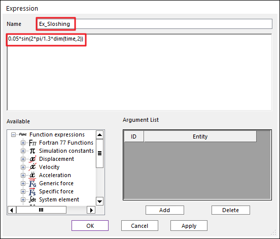
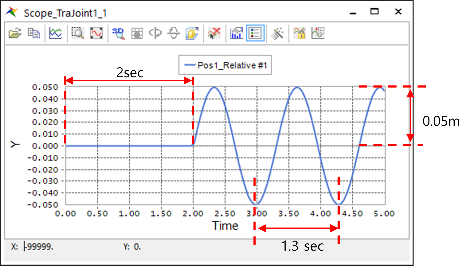
   The expression creates a motion of the translational joint as shown in the figure below, with an amplitude of 0.05m and a period of 1.3 seconds starting from 2 seconds. The initial delay of 2 seconds is used for the purpose of allowing the fluid particles in the tank to settle before the forced oscillations begin.

   

8. Click OK to close all the dialog boxes.

Now you have completed the creation of the all necessary RecurDyn elements for a simulation that does not include co-simulation with Particleworks. Next, you will create what is called a Wall in RecurDyn, which is required for co-simulation with Particleworks.

10.1.3.6. Creating the Wall

Next, you will create a Wall on the Container body you just created.

1. From the Particleworks group in the External SPI tab, click the Walls function.

2. Click the Container.Shell1 on the Working Window as solid.

   Note

   What is Wall?

   A Wall is a rigid body surface in a RecurDyn model that can make contact with the fluid in Particleworks during co-simulation. The Wall is the primary element of interaction between RecurDyn and Particleworks.

   RecurDyn passes the positions and velocities of the Wall surfaces to Particleworks. In Particleworks, the surfaces can make contact with the fluids. Particleworks computes the forces of interaction between the surface and the fluid. These forces are then sent back to RecurDyn to influence the motion of the body to which the Wall surface is attached.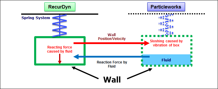

   

10.1.3.7. Exporting the *.wall

1. From the Particleworks group in the External SPI tab, click the Export function.

2. Display the dialog box to save the file by clicking OK.

   The rd_pw.wall file and WallGeometries folder are created in saved folder. These will be moved to the Particleworks project folder created in chapter 4.

   Note

   In the WallGeometries folder, the geometry files (*.obj or *.stl) for Wall is saved. And in the rd_pw.wall file there is information about the position of each wall geometries.

10.1.3.8. Analyzing the RecurDyn Model

10.1.3.8.1. Executing the Simulation Without Co-Simulation:

Before running the co-simulation between RecurDyn and Particleworks, you may want to verify that the model which you just created works properly. Since RecurDyn will automatically run co-simulation with Particleworks when there is a Wall in the RecurDyn model, you should change several options to allow RecurDyn to execute the simulation without co-simulation with Particleworks.

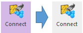
1. From the Particleworks group in the External SPI tab, inactivate the Connect function.

   

2. From the Simulation Type group in the Analysis tab on the main RecurDyn ribbon control, click the Dynamic / Kinematic Analysis function.

3. Enter the following:

   • End Time: 14

   • Step: 1400

4. Click Simulate to analyze.

10.1.3.8.2. To display an animation of the simulated motion:

• After the completion of analysis, click Play on the Analysis tab of the main RecurDyn ribbon control to view the animation.

• You can animate the Container body moving from side to side. The modeling in RecurDyn has been completed. Now you will exit RecurDyn after saving the model, then proceed to modeling in Particleworks.

10.1.4. Creating a Model in Particleworks

Fluids are modeled in Particleworks using a particle method, where each particle represents a certain mass of fluid. Creating a model in Particleworks involves defining a collection of these fluid particles. There are various methods for defining the particles in Particleworks. In this tutorial, you will use the method of filling particles from the defined plane to the boundary surface of a Wall.

10.1.4.1. Task Objective

Learn how to create fluid particles, enter a property of matter, and configure the analysis environment.

10.1.4.2. Estimated Time to Complete

15 minutes

10.1.4.3. Starting Particleworks

10.1.4.3.1. To create a new model:

1. On your Desktop, double-click the Particleworks icon.

2. Click Create Project from the File tab. Display the Create Project dialog box.

   

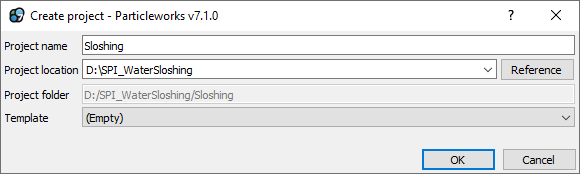
3. Enter Sloshing for the name of the Project Name.

4. Specify the folder in which the project files will be created in Project Location.

5. Click Finish, and then Particleworks will create the new model that you specified.

10.1.4.3.2. Copy the RecurDyn files:

The RecurDyn model and Wall files should be manually copied into the Particleworks project folder for co-simulation.

• You must move the Sloshing.rdyn file, rd_pw.wall file, and WallGeometries folder which you just created in chapter 3, to the scene folder for the Particleworks project.

• (Folder path: <ProjectLocation>\Sloshing\scene)

10.1.4.4. Setting up the Pre-process

Pre-process is the process to define the overall system of modeling from the particle creation to the environment settings.

10.1.4.4.1. To import the Wall from the Wall file:

1. Click scene from the Projects dialog.

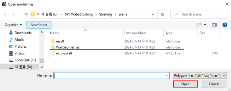
2. Click the Import polygon files icon to import rd_pw.wall file. Open model files dialog is displayed.

3. Select Rd_pw.wall file, and click Open. (<ProjectLocation>\Sloshing\scene\rd_pw.wall)

   

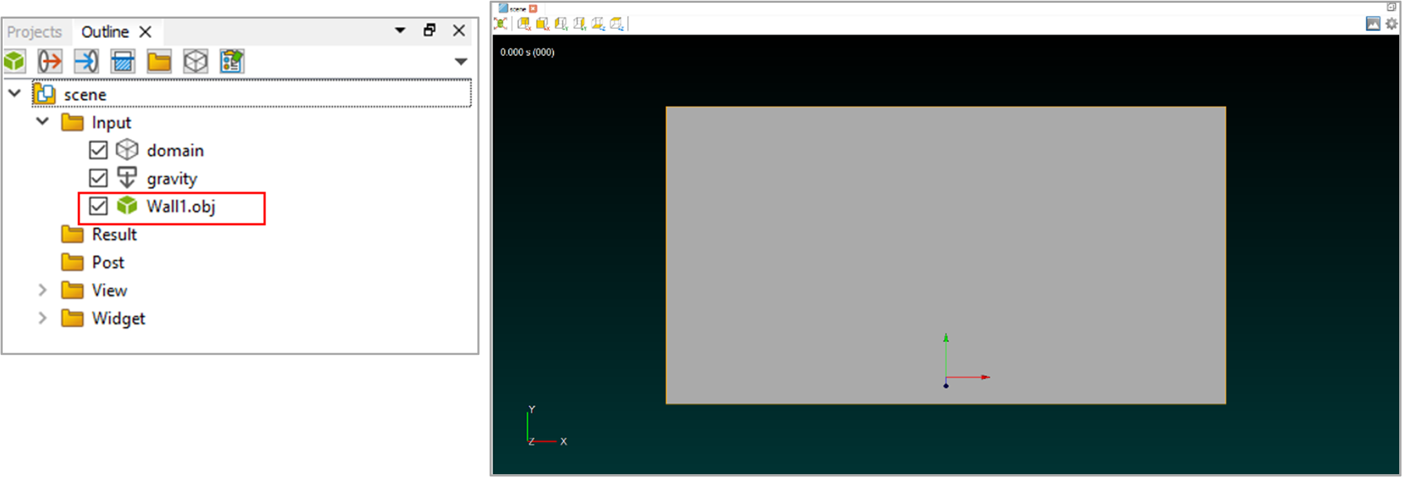
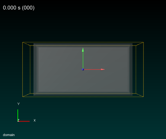
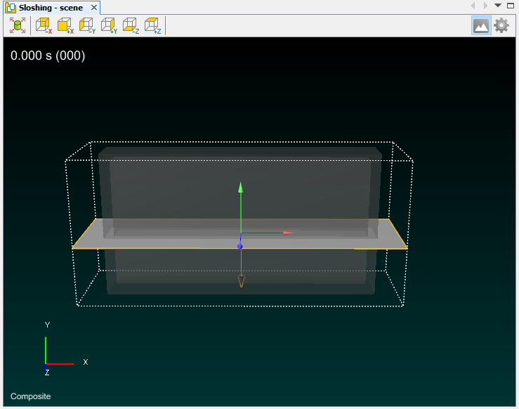
4. Click Fit and +Z to take a close look at the Wall which you just imported.

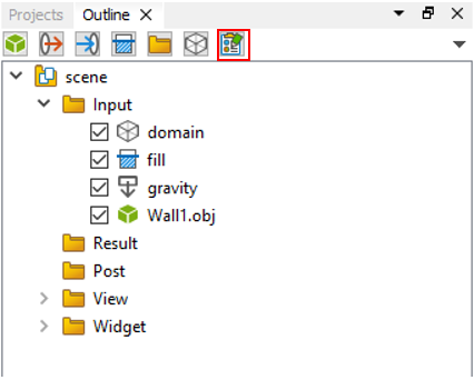
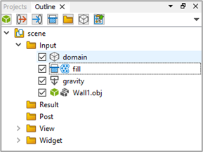
   If the Wall has been properly imported, then an item titled Wall1.obj will be visible in the database tree under Sloshing > scene > Input, as shown in the figure below. The imported Wall should be visible in the Working Window as well.

   

10.1.4.4.2. To set the transparency of a Wall:

It is recommended that you set the Wall1.obj object to be transparent. This will be useful when creating the fluid particles.

1. Click Wall1.obj on the Projects dialog box (scene > Input).

   Display the Properties dialog box about the entity you have clicked below scene tree.

2. Change Alpha to 0.3 under the Appearance and press the enter key.

   

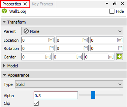
   You can see that the Wall1.obj object becomes transparent.

10.1.4.4.3. To set the domain:

The Domain in Particleworks signifies absolute volume of space in which the fluid particle can be permitted to move during the fluid simulation in Particleworks. This volume should include the entire volume of space that the Wall1.obj object is expected to pass through during the simulation. It is acceptable for the Domain volume to be larger than the volume through which the Wall1.obj actually passes through during the simulation.

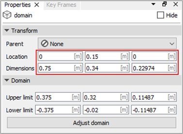
1. Click on domain in the Projects database tree. (Sloshing > scene > Input)

2. Enter the following in the Location under the Transform.

   • Location: 0, 0.15, 0

3. Enter the following in the Dimensions under the Domain.

   • Dimensions: 0.75, 0.34, 0.22974

10.1.4.4.4. To create the particles:

Fill has a function of filling both the defined plane and closed space of Wall1 with particles. The plane is limited to the inside of the domain.

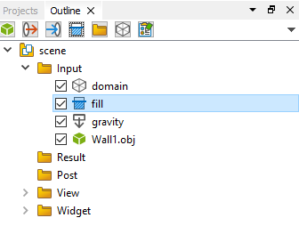
1. Click Fill in the PW Wizard dialog box.

   An item titled Fill will be created in the Projects database tree. (Sloshing > scene > Input)

   

2. Click Fill in the Projects database tree.

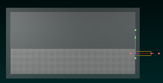
3. Enter the following under the Transform in the Properties dialog box.

   • Location: 0, 0. 12, 0

   • Direction of Particle Creation: yLower

     

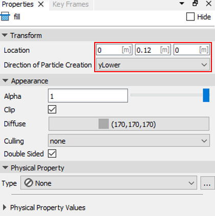
4. Confirm that Fill is defined as shown in the figure below.

   

10.1.4.4.5. To create and set the physical properties of the fluid:

1. Click Manage physical properties… icon to create the property of matter upper scene tree. The Physical property manager dialog box appears.

   
2. Click + to create Fluid.

   The default properties are the physical properties of water. Use these properties for the tutorial model.
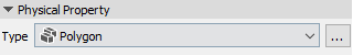
3. Click + to create Polygon.

   Polygon is used to define the material properties of the contact surface of the Wall1.obj object.
   

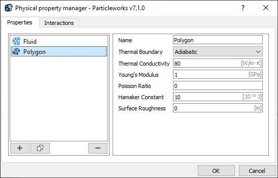
4. Click OK to exit the Physical property manager dialog box.

5. Enter the following in the Physical property in the Properties dialog from None to:

   • Wall1.obj: Polygon

   • Fill: Fluid

   

10.1.4.4.6. To configure the particles and environment:

You will change the options of Basic tab in the Run dialog box clicking Setting icon.

1. Enter 0.005 in the Particle Size.

   

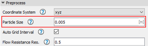
2. Enter -9.8 in the Y of Gravity, the same value with RecurDyn.

   

3. Click Next, and enter the following under the Pressure in MPS tab:

   • Type: Implicit

4. Select the Explicit option under the Viscosity.

   

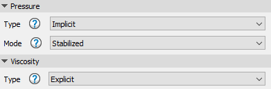
5. Click Next to go to the next page.

10.1.4.4.7. To configure the analysis conditions:

You will change analysis options in the PW Wizard dialog box.

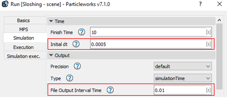
1. Enter 0.0005 in the Initial dt[s] under the Time.

   The above value signifies the initial step size and the maximum step size. It also performs same role as Initial Time Step and Maximum Time Step in RecurDyn.
2. Enter 0.01 in the File Output Interval Time[s] under the Output Settings.

   The above option value signifies time (second) interval between steps. This value should be identical with that of EndTime/Step in RecurDyn.
   

10.1.4.4.8. To create the particles:

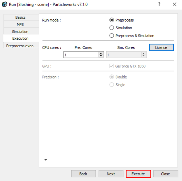
1. Click Execute after completing the simulation configuration. Display the Run dialog box.

2. In the category Run mode, select the radio button Preprocess.

3. Click Execute.

   

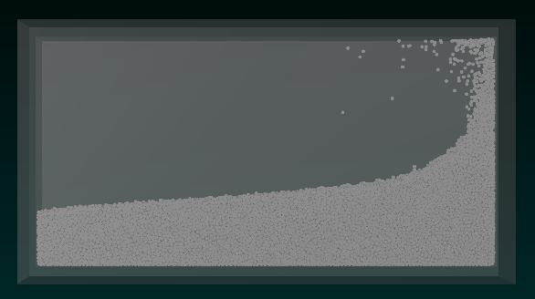
   The fluid particles in the Wall1.obj object will be created after clicking the Execute button. They should look like the image. A message will be displayed in Working Window of tasks tab

   The necessary files for co-simulation will be created in the df, pre folders in the project folder (<ProjectLocation>\Sloshing\scene) during the analysis.

10.1.4.5. Preparing for Co-Simulation with RecurDyn

A number of files that are generated by Particleworks are required by RecurDyn for the co-simulation of RecurDyn with Particleworks. These files are automatically generated by Particleworks when Particleworks executes a simulation independent of RecurDyn. Therefore, it is required that you run a simulation first in Particleworks using the model that you have just created, but without co-simulation with RecurDyn.

10.1.4.5.1. Simulation in Particleworks Independent of RecurDyn:

1. Click Run in the Simulation tab. The Run dialog box appears.

2. In the category Run mode, select the Simulation radio button.

3. Enter the number of CPU cores that you wish to use during this simulation.

   Compatible GPUs for your computer will be listed in the GPU category on this page of the Run dialog box. If you wish to use one of the GPUs for this simulation, select the GPU from this list.
   

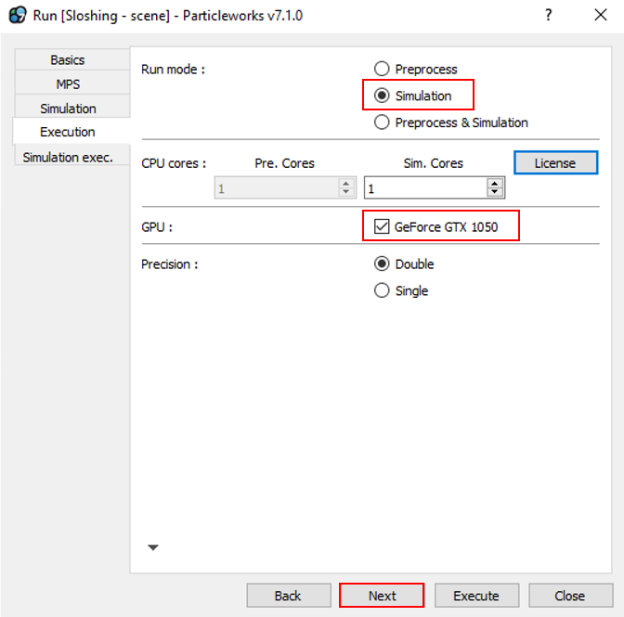
4. Click Next.

5. Click Close without running simulation radio button.

   

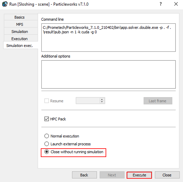
6. Click Execute.

   All the necessary files for co-simulation will be created in the result folder in the project folder (<ProjectLocation>\Sloshing\scene) during the analysis

   Now you are ready for co-simulation between RecurDyn and Particleworks.

7. Save the project.

It is not necessary to run Particleworks while you are working on chapter 5. But in the next chapter, you should run Particleworks to check the result in real time.

10.1.5. Co-Simulation

In this chapter, RecurDyn and Particleworks will run co-simulation for behavior analysis between rigid bodies and particles.

10.1.5.1. Task Objective

Learn how to run co-simulation in RecurDyn.

10.1.5.2. Estimated Time to Complete

120 minutes

10.1.5.3. Co-Simulation

10.1.5.3.1. To run co-simulation in RecurDyn:

1. Start RecurDyn and open Sloshing.rdyn file which you just copied in chapter 3.(File path :<ProjectLocation>\Sloshing\scene\Sloshing.rdyn)

2. From the Particleworks group in the External SPI tab, activate the Connect function.

   

3. From the Simulation Type group in the Analysis tab of the main RecurDyn ribbon, click the Dynamic / Kinematic Analysis function.

4. In the Parameter page, enter 1.e-003 in the Maximum Time Step input field.

   

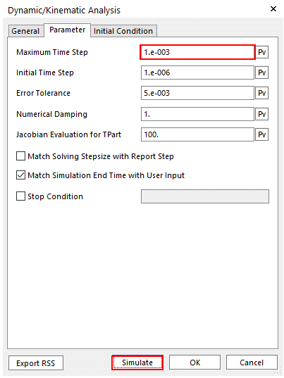
5. Click Simulate.

   RecurDyn will start a co-simulation with Particleworks. (The estimated time depends on the specifications of both CPU and GPU.)

Tip

Set RPA Setting option in Particleworks Setting dialog

Before proceeding co-simulation, user needs to use TranslationalVelocity, the data of RPA file, which is the output of the particle, for contour.

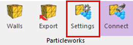
• Click the Settings function in External SPI tab.

  

• Check Use option of TranslationalVelocity in RPA Settings.

  

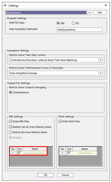
• Click OK.

10.1.5.3.2. To view the progress of analysis:

You can view the progress of analysis of the fluid particles being simulated in Particleworks through the Particleworks GUI.

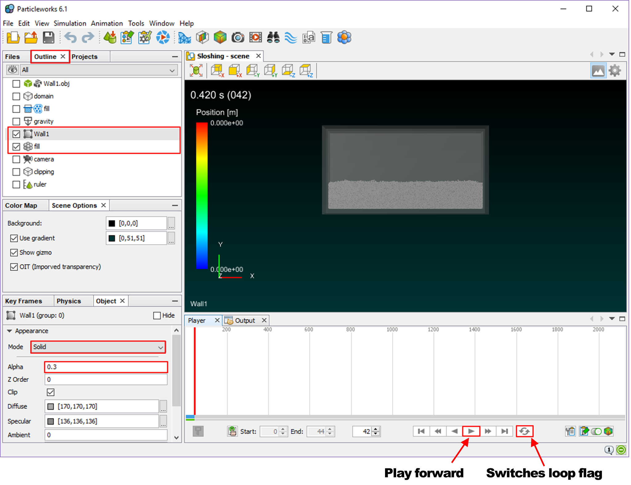
1. Select the Wall1 and fill checkboxes in the Outline dialog box.

2. Click the Wall1 in the Outline dialog box.

3. Change the below options in the Object dialog box of Wall1.

   • Mode: Solid

   • Alpha: 0.3

4. Turn off the Switches loop flag option in the Player dialog box.

   The Switches loop flag option is for endless loop of animation.
5. Click Play forward in the Player dialog box.

   You can view the animation of completed time steps up to the present time.
   

10.1.5.4. Working with Animations

10.1.5.4.1. To play an animation:

• From the Animation Control group in the Analysis tab, click the Play / Pause function.

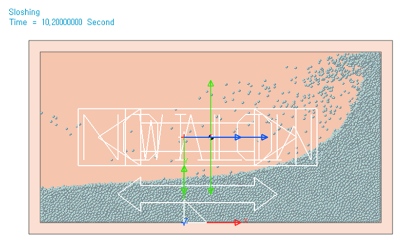
The Wall motion results in both the generating of reaction force and the particle behavior by the impact between the particles created inside of the Wall and the inside walls of the Wall. In the beginning of area of shaking the Wall, the period form of particles is irregular. But you will notice that the particles gradually start moving with a regular period form as the cycle is repeated several times.

10.1.5.4.2. To display a particle contour:

Color can be used to display various properties of the fluid during the animation.

1. From the Post-Process group in the External SPI tab, click the Particle Contour function.

2. Change the Contour Type to Translational Velocity Magnitude.

3. In the Min/Max Option, set Min/Max values.

   • Min: 0.1

   • Max: 1

4. Uncheck the Show Min Value and the Show Max Value.

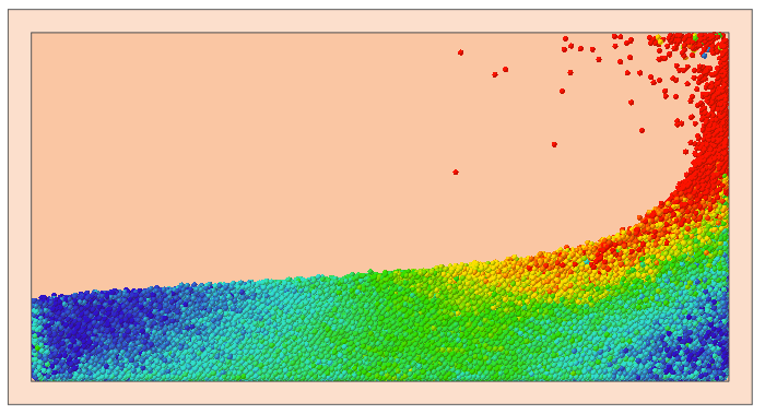
5. Check the Enable Contour View and click OK.

   

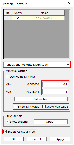
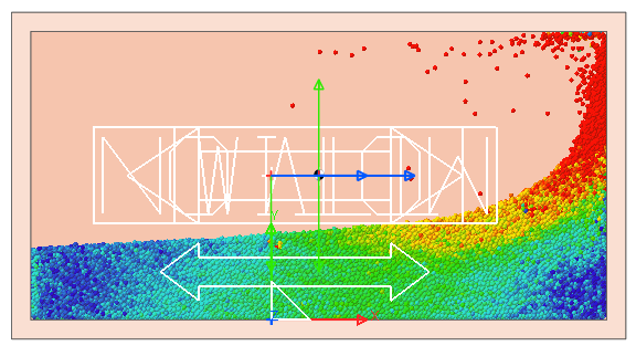
   Now you have set contour to display the particles using colors to represent particle speeds relative to the reference coordinate system, as shown in the figure below.

   

10.1.5.5. Working with Plots

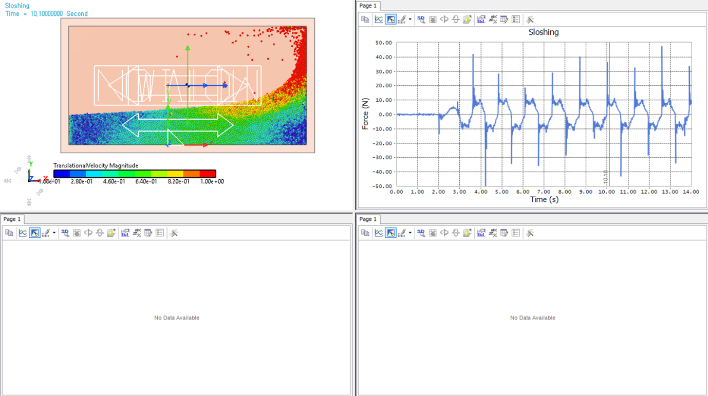
You will see the cyclic fluid forces in RecurDyn acting on the tank body for caused by the sloshing of the fluid.

10.1.5.5.1. To view the driving torque:

1. From the Plot group in the Analysis tab of the main RecurDyn ribbon, click the Plot Result function.

2. From the View group in the Home tab of the ribbon, click the Show All Windows function.

3. From the Animation group in the Tool tab, click the Load Animation function in the upper left side of the window.

4. Plot the FX_Reaction_Force of the Wall1 in the upper right side of the window.

   The result should look like the figure below. In the plot on the right, the reaction force acting in the x-direction on the body Wall1 can be seen. The reaction force has a repeating cyclic shape that matches the animation shown in the left window.
   

10.1.6. Particleworks Postprocessing

In this chapter, you will use Particleworks to calculate fluid pressure and create an animation of fluid behavior by utilizing post-processing functionality in Particleworks.

10.1.6.1. Task Objective

Learn how to view the results of the fluid simulation and how to create a surface which looks like an actual fluid.

10.1.6.2. Estimated Time to Complete

30 minutes

10.1.6.3. Working with Animations

You can view the animation of analysis result in Particleworks.

10.1.6.3.1. To play an animation:

• Click Play to view the animation.

10.1.6.3.2. To create the probe:

A probe is a particle whose result data can be plotted. You will create a probe and then plot the pressure experienced by that particle during the simulation.

1. Click Probe in the Tools tab. The Probe dialog box appears on the below side.

   

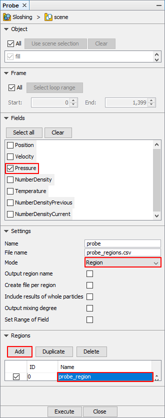
2. Select Pressure under the Fields.

3. Set Mode to Region under the Settings.

4. Click Add under the Regions.

5. Click the list of ID 0 the Name is prove_region.

   The Object dialog box for probe_region appears on the below side.
   

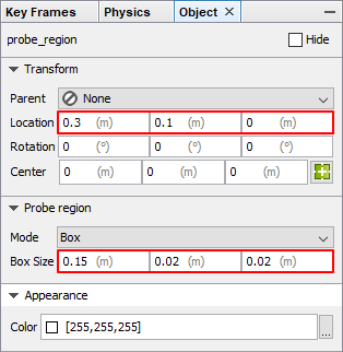
6. Enter the following under the Transform in the Object dialog box.

   • Location: 0.3, 0.1, 0

7. Enter the following under the Prove region in the Object dialog box.

   • Box Size: 0.15, 0.02, 0.02

   Now you have created the probe within the bounds of motion to measure the wall on the right side of the Wall.

   

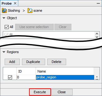
8. Click Execute.

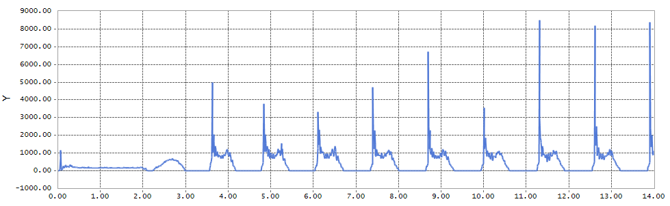
   The probe result has been created as a CSV file type. The folder where the file is saved will appear following the completion of the CSV file creation.

   (Folder path: <ProjectLocation>\Sloshing\scene\prove)

The CSV output file can be opened by any appropriate program, such as Microsoft Excel, to view and plot its contents. The figure below was generated by Excel. It shows a plot of the pressure of the probe particle over time.

• X : SimulationTime

• Y : Pressure_max

10.1.6.4. Creating the Surface

You can create a smooth surface of fluid behavior presented like as actual surface in Particleworks.

10.1.6.4.1. To create the surface:

1. Click Surface generator in the Tools tab. The Surface generator dialog box appears on the below side.

   

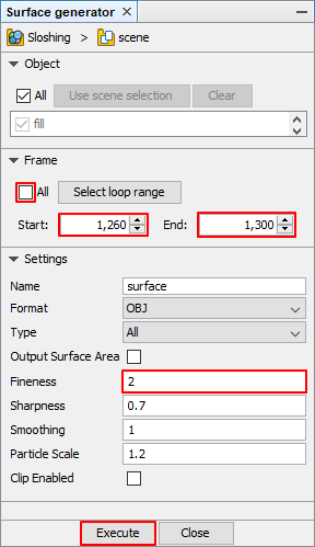
2. Enter and check the following in the Surface generator dialog box.

   • Start Frame: 1260

   • End Frame: 1300

   • Fineness: 2

3. Click Execute. You can check the current situation of progress in the Output dialog box.

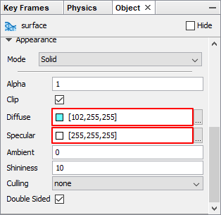
4. Double-click surface in the Project dialog box after completion of surface creation. (scene > Post)

5. Change the values of Diffuse and Specular in the surface options as below.

   • Diffuse: 102, 255, 255

   • Specular: 255, 255, 255

     

10.1.6.4.2. To hide the particle animation:

You should hide the existing particles of animation in Particleworks through the Particleworks GUI.

• Turn off the fill checkbox and select the surface checkboxes in the Outline dialog box.

  

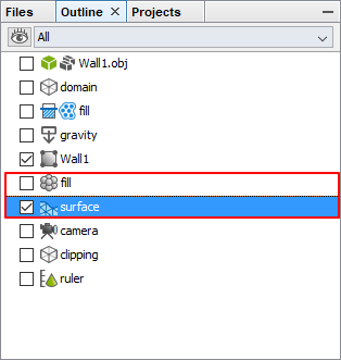
You will see the result as shown in the figure below when playing the animation again.

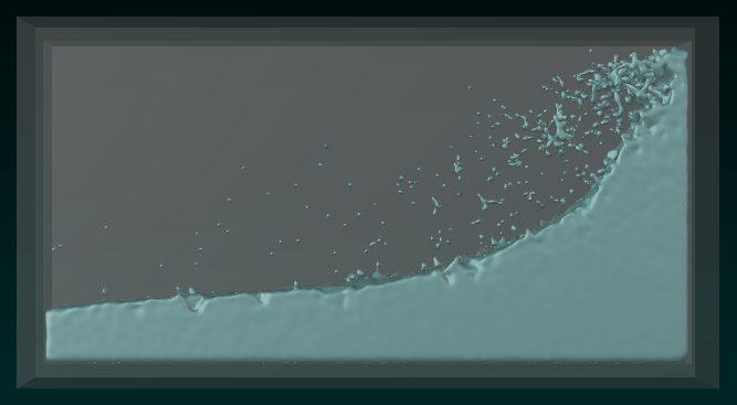
In the period step1260 to step1300, this animation shows the result close to the flow of actual fluid by creating the smooth surface. Your presentation and report writing will be more convincing by using the images and animations created by this function.

10.1.7. Result Analysis and Review

10.1.7.1. Task Objective

Learn how to do a comparative analysis between the trial result value from paper and the analysis result value from co-simulation between RecurDyn and Particleworks.

10.1.7.2. Estimated Time to Complete

5 minutes

10.1.7.3. A Comparative Analysis of Results

You will judge the reliability of the MPS analysis method by doing a comparative analysis between the result from reference paper and the trial result according to this tutorial.

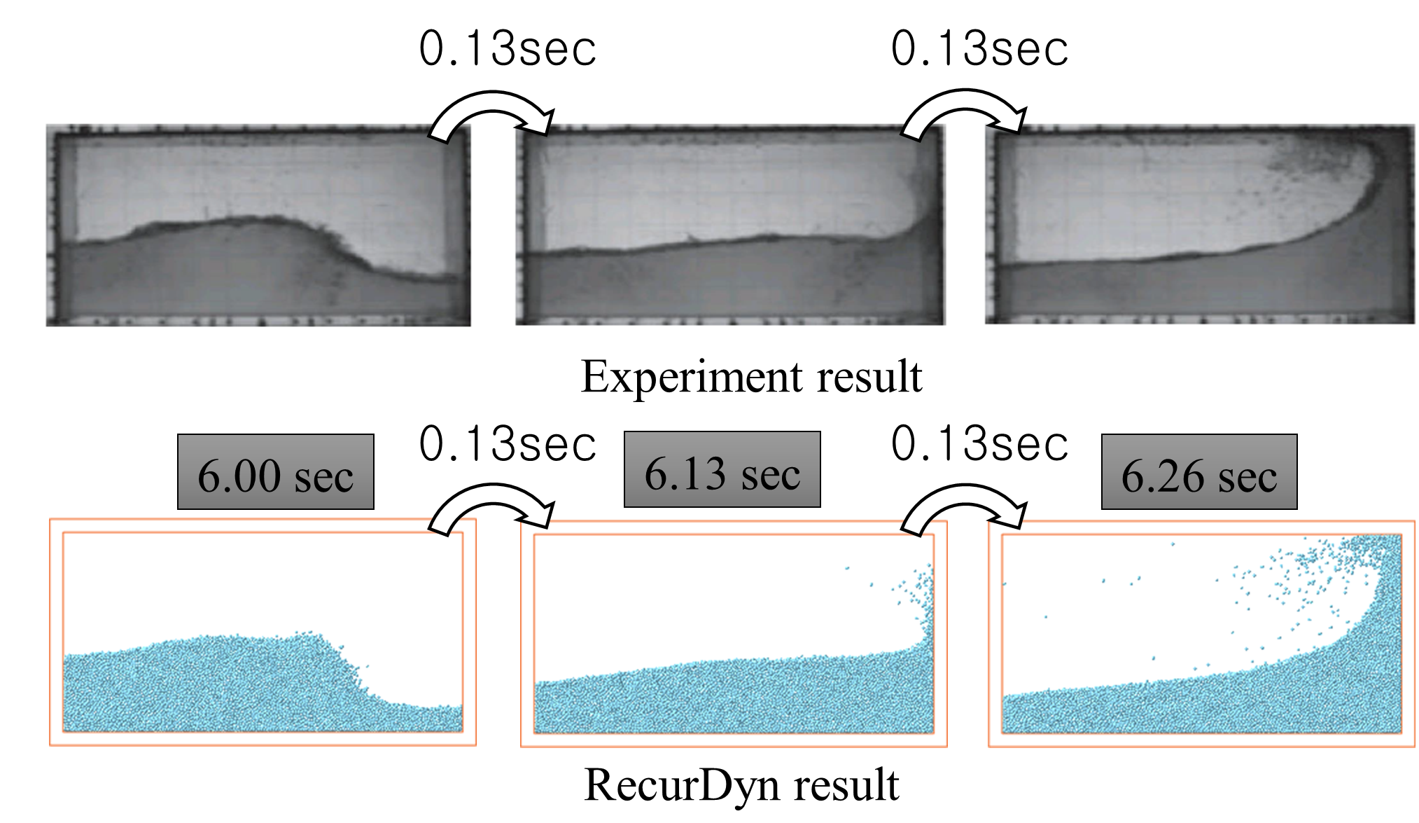
10.1.7.3.1. A comparative analysis of fluid behavior results:

The figure below shows the profile of fluid behavior at intervals of 0.13 second. As you can see in the figures below, the fluid waveform created from the left side breaks hitting against the wall while moving to the right. The analysis result from trial shows that the waveform started moving to the right breaks hitting against the wall presenting the same waveform as the profile of trial.

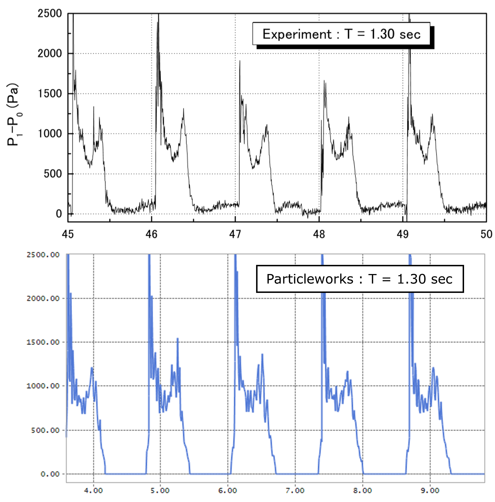
10.1.7.3.2. A comparative analysis of fluid pressure result:

The figure below, as a pressure graph against time, shows both the data extracted from the trial and the data gained from the analysis from chapter 6 in this tutorial. Both pressure data values are measured under the same condition of 10cm above the ground.

Through a comparative analysis of two graphs, the similar pressure values in the similar pattern are created at the moment when the fluid hits against the wall with the periodic motion of 1.3 seconds.