3.6. Landing Gear System Tutorial (AutoDesign)

3.6.1. Landing Gear System Design Problem

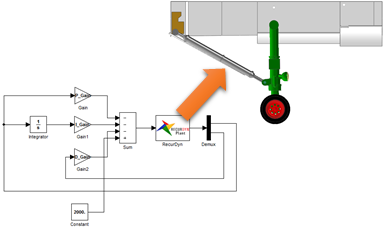
RecurDyn provides the CoLink module that is used to model a control system. If you use CoLink in RecurDyn, you will make an approximate model for control system. That means that the CoLink can directly control the RecurDyn model. Thus, if the RecurDyn model is fully validated, this approach can be a virtual control system. Suppose that a PID controller system controls the actuating force of a landing gear system. The goal of controller is to move the wheel into the bay and make it to be stable in 2 seconds.

As the CoLink directly uses the Parametric Values defined in RecurDyn, all gain values can be defined by using the parametric values. Also, the goal of control system can be represented by the Expressions. Thus, AutoDesign can find the optimal gain values easily to satisfy the goal of control system.

Open files related in Sample-F
Sample	1	<InstallDir>\Help\Tutorial\AutoDesign\AutoDesign_F\Examples\Sample_F.rdyn
	2	<InstallDir>\Help\Tutorial\AutoDesign\AutoDesign_F\Examples\Sample_F.clk
Solution	1	<InstallDir>\Help\Tutorial\AutoDesign\AutoDesign_F\SolutionsSample_F.rdyn
	2	<InstallDir>\Help\Tutorial\AutoDesign\AutoDesign_F\Solutions\Sample_F.clk

Note

If you change the file path at discretion, it can be located in any folder that you specify.

3.6.2. Loading the Model and Playing a Control System

3.6.2.1. To load the base model and view the animation:

1. On your Desktop, double-click the RecurDyn software. RecurDyn starts and the Start RecurDyn dialog box appears.

2. Close Start RecurDyn dialog box. You will use an existing model.

3. In the Quick Access Toolbar, click the Open and select Sample_F.rdyn from the same directory where this tutorial is located. The landing gear system appears on the window.

   

4. In the Communicator tab, click the Run CoLink function. Then, the CoLink appears. In the toolbar, click open tool and select Sample_F.clk from the same directory where Sample_F.rdyn is located.

   

5. Click Start in the CoLink.

6. Click Play in the RecurDyn.

The landing gear system moves into the bay. If not, the CoLink model is not connected to RD model. Retry to load CoLink Model or push the Connect CoLink button on CoLink

3.6.3. Defining the design variables

The design variables are the gain values of PID controller. Thus, create the three parameters and define the initial values.

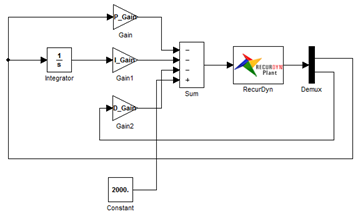
Switch the window to CoLink window. Then, the three parameters are shown in the data base window. Next, you can link the parametric variables to P, I, and D gains, which is shown by the following figure.

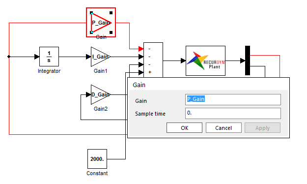
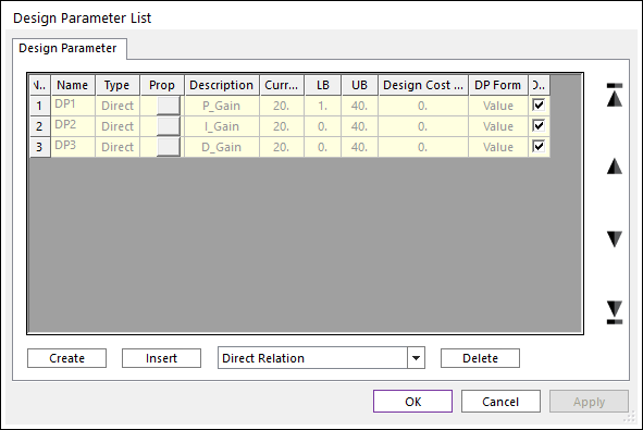
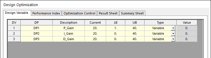
Now, click the Design Parameter function and link the three parametric variables to the design parameters. The lower and upper bounds are arbitrarily selected except the P-Gain. In general, as P-Gain should be used conceptually, its lower bound is set to 1.

3.6.4. Defining the Analysis Responses

The Plant represents the system model to be controlled. Thus, the Plant Input is the output of the controller and the Plant Output becomes the input responses for the controller.

In this model, the Plant Input is the axial force of the nose gear strut and the Plant Output is the relative position and the relative velocity between the wheel center and the target position along the vertical direction.

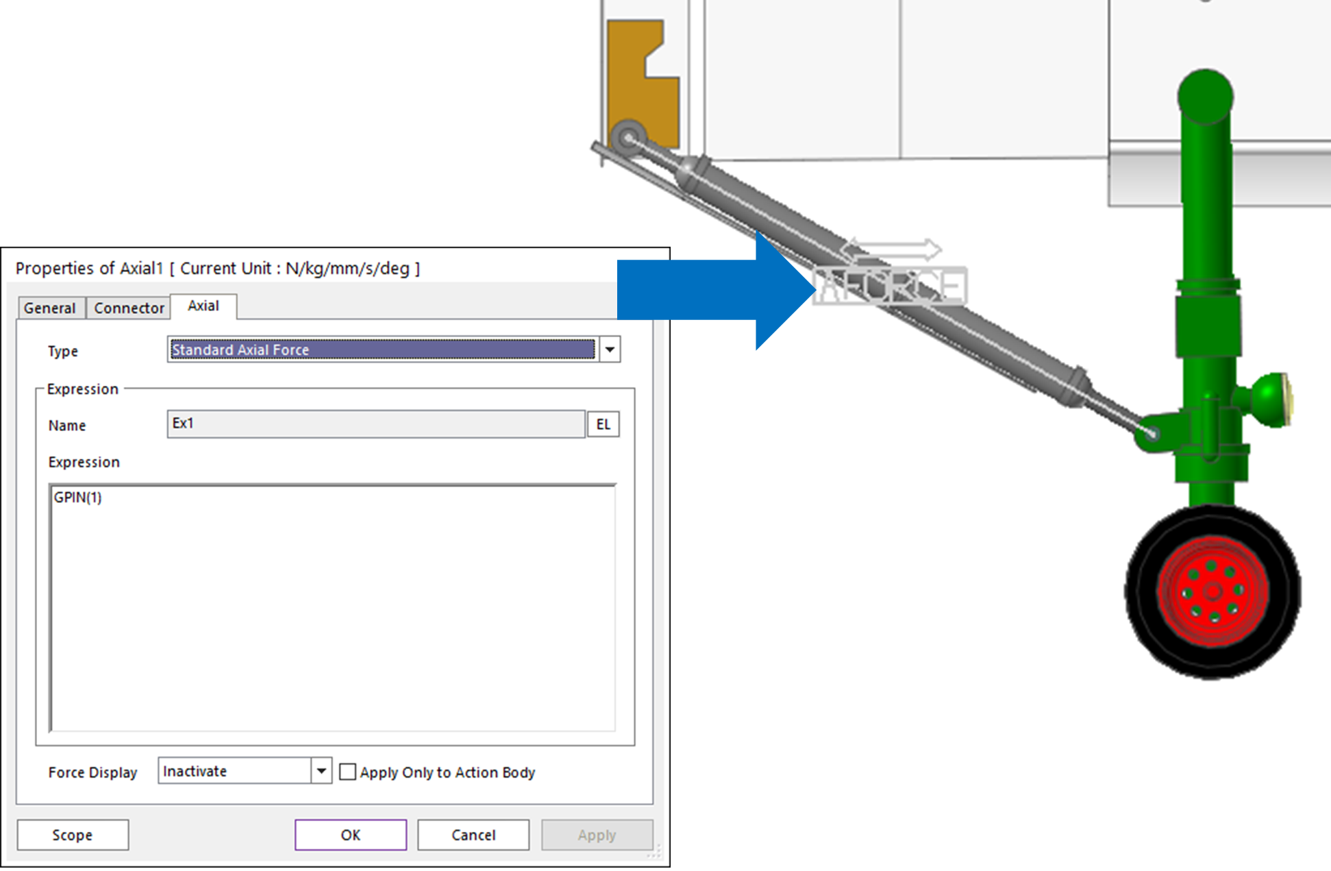
In order to link the Plant Input to the axial force, first, the Plant Input is represented by the Expression. Next, the Expression is used to define the axial force.

Also, the Expression is required to define the Plant Output. For more information of CoLink, refer to the CoLink manual.

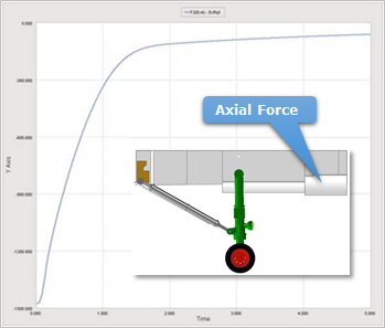
The goal of controller is to minimize deviation between the wheel center and the target position in 2 second. The initial gain values give the following result. The deviation is not zero in 5.0 second.

Now, let’s consider the design optimization problem:

Minimize the deviation in 2.0 second to satisfy the goal of controller.

For safety, the maximum transient response of the deviation should not hit the upper wall of the bay.

For manufacturing, the Plant Input should be less than a limit value.

Although the deviation is minimized, it is not guarantee that the value goes to zero. Thus, in order to enforce the deviation, go to zero, the following additional constrain is introduced.

The end value of the deviation should be zero.

Let’s consider the Expression to represent the design formulation and define the Analysis Responses.

1. Define the deviation by using the Expression. The STEP function is used to filter the values only in 2.0 second.

2. List the Expression. Among the Expressions, Ex1 is the Plant Input. Ex4 is the deviation between the wheel center and the target position. Ex5 is the filtered response of Ex4.

3. Next, create the Analysis Response as follows:

   The detailed information between ARs and Expressions are listed as:

   AR name	Expression name	Treatment
   AR1	Ex4	Max Value
   AR2	Ex1	Max Value
   AR3	Ex5	Max Value
   AR4	Ex4	Max Value

3.6.5. Running a Design Optimization

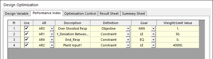
The optimization problem is defined as:

Minimize the RMS of the Deviation

subject to

• The Maximum Peak of Transient response of the Deviation =< Limit value

• The Plant Input =< Limit Value

• The end value of Transient response of the deviation = 0

1. Click the Design Optimization function. Then, you can see the design variable list as below figure:

   

2. Click the Performance Index page. Then, you can see the following list. If this window is empty, then you create the following PI s.

   

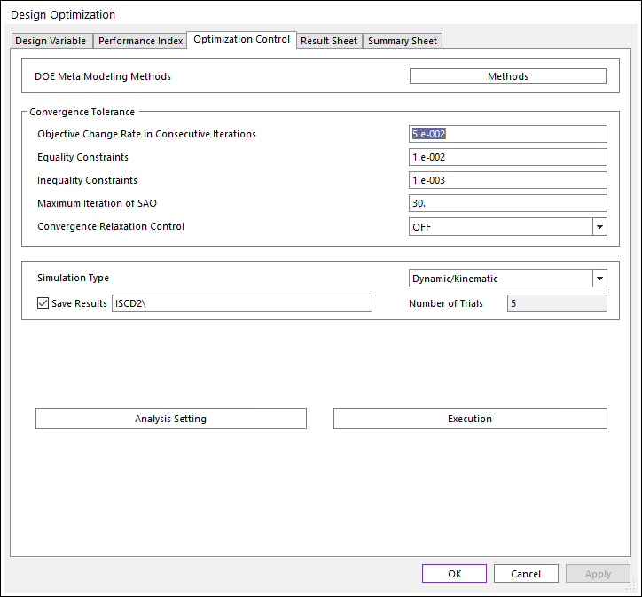
3. Click the Optimization Control page. All the convergence tolerances use the default values. It is important to check the time step in Analysis setting before clicking Execution. Especially, when the CoLink is used, the sampling time step of dynamic analysis is equal to that of the CoLink.

   

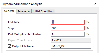
4. Click Analysis Setting. Then, you can see the following information. The End time is 5 second and the number of Step is 500. Thus, The Expression values are nearly evaluated at the time interval of 0.01 second.

   

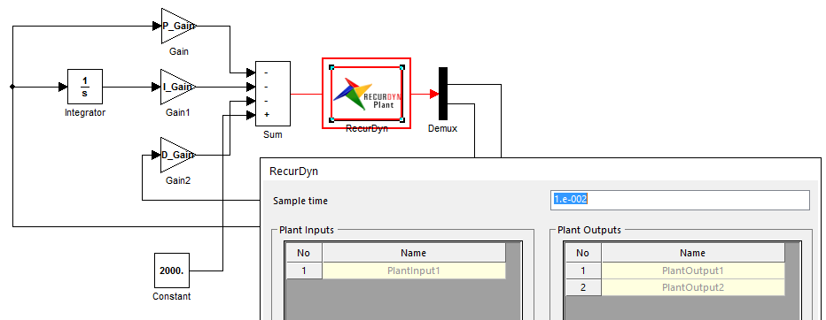
5. Switch the window into the CoLink. Then, double click the RecurDyn Plant. Then, the sample time appears in the pop-up window. Both sample time should be equal. For more information, refer to the CoLink manual.

   

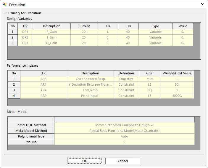
6. Click Execution. Check the Execution dialog box. If all selections are correct, then click OK.

   

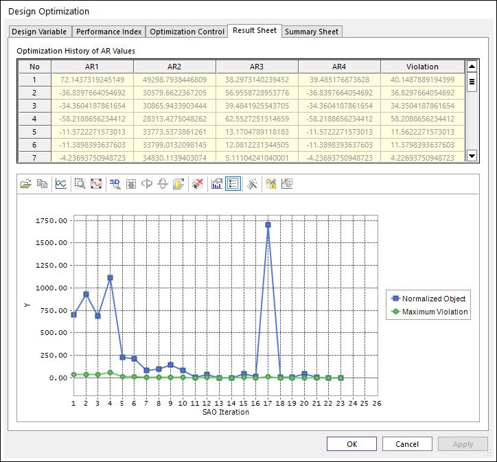
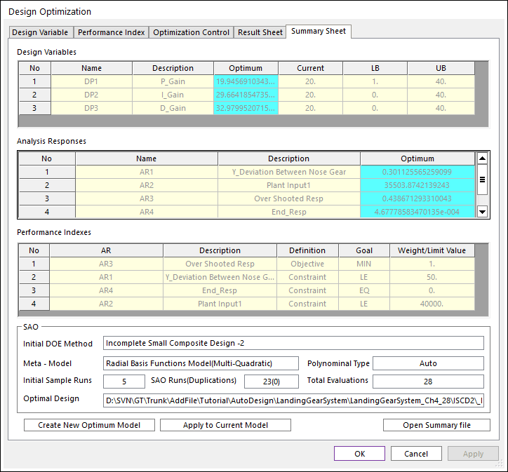
7. If the optimization is completed, then click the Result Sheet page. The optimization runs 20 iterations. The final values of ARs are (9.702, 36364.52, 1.0998, -5.188e-002). The number of total analyses is only 25 including the initial sampling analyses. Next, see the Summary Sheet.

   

3.6.6. Comparison of analysis results

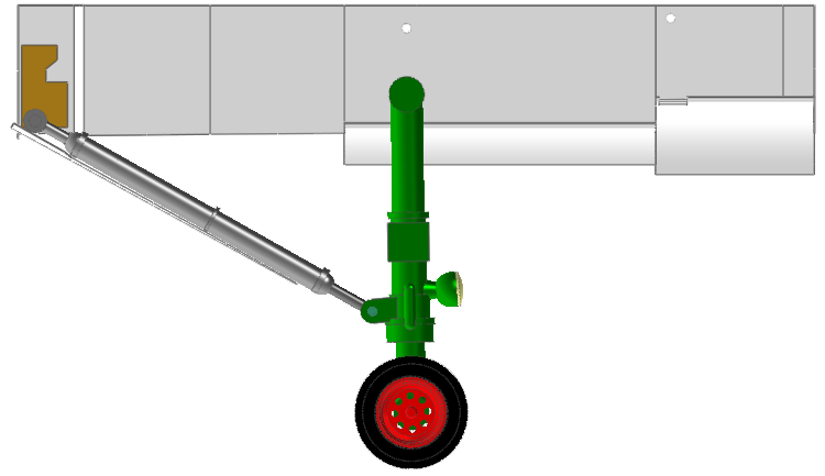
Let’s compare the animations for the initial and the final design. The initial design uses the gain values as (20, 20, 20). The final design gives an optimal gain value set as (13.89, 34.24, 24.28). Figure 3.52 shows the animation result for the initial design.

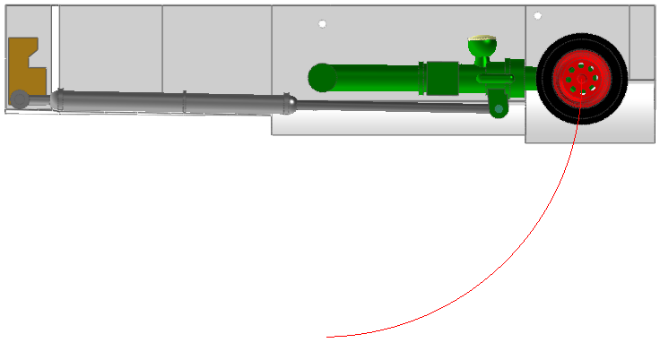
Figure 3.52 The animation result for the initial design

Next, Figure 3.53 shows the animation result for the final design. This design moves the wheel center position more up than the initial one.

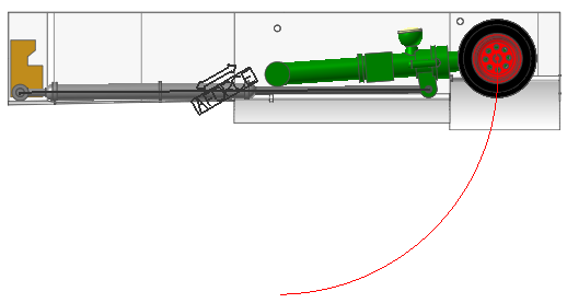
Figure 3.53 The animation result for the final design

Figure 3.54 compares the deviation responses for the initial design and the final design. The red line is the final design. The blue line is the initial design. After 2.0 second, the final design makes the deviation to be zero.

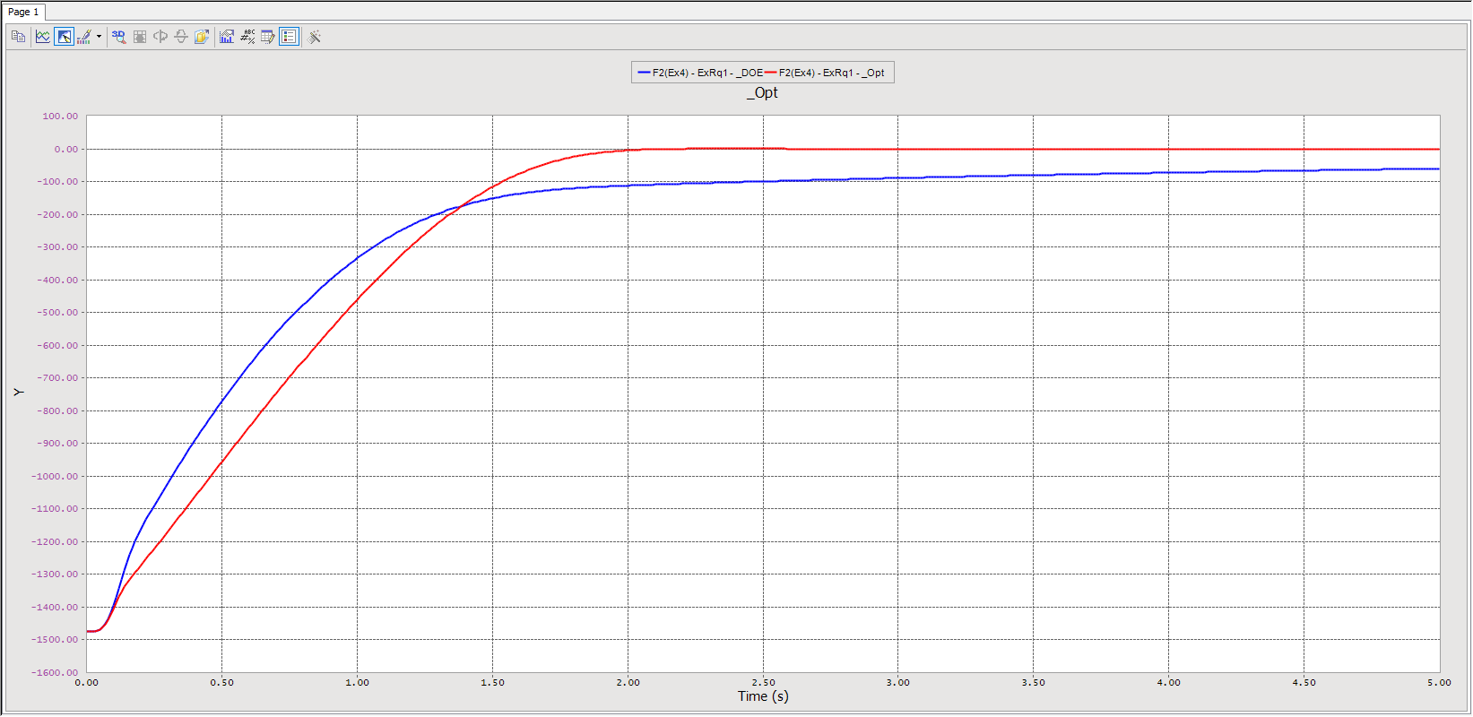
Figure 3.54 Comparison of the deviation responses