11.3. Macpherson Strut Design Study Tutorial (eTemplate)

11.3.1. Overview

There are Creation Mode and Modification Mode for the modeling methods by the eTemplate. And Plot Automation is used for reporting the results.

• Creation Mode allows you to start a new model or open an existing model and create a new entity.

• Modification Mode allows you to define the entities in a model using a template and change the parameters to modify the model.

• Plot Automation allows you to define the axis information and data for the curve using an Excel template so that you can plot data easily and repeatedly.

Generally, once you finish a model and complete the final step, you want to simulate the model by changing a few parameters repeatedly. At this time, you may need to draw the results repeatedly using the same type of graph. You can use the Modification Mode and Plot Automation functions of an eTemplate to automate these repeated processes.

11.3.1.1. Task Objectives

This tutorial includes the following tasks:

• Creating and running a Modification Mode template

• Creating and running a Plot Automation template

11.3.1.2. Prerequisites

• This tutorial is intended for users who have completed the RecurDyn basic tutorial. If you have not completed the tutorial, then you should complete it before proceeding with this tutorial.

• You need Microsoft Office Excel (2007 or above) to process this tutorial.

11.3.1.3. Procedures

This tutorial consists of the following tasks. The following table outlines the time required to complete each task.

Procedures	Time (minutes)
Sample Model Study	10
Run Modification Mode	20
Run Plot Automation	20
Total	50

11.3.2. Sample Model Study

11.3.2.1. Task Objectives

This chapter explains the sample model provided in this tutorial and the entity parameters available in Modification Mode.

11.3.2.2. Estimated Time to Complete

10 minutes

11.3.2.3. Opening the Sample Model

11.3.2.3.1. To run RecurDyn and open the initial model:

1. Run RecurDyn. The Start RecurDyn dialog window appears.

2. Click Browse.

3. In the eTemplate tutorial directory (<InstallDir>\Help\Tutorial\eTemplate\ModificationMode\MacphersonStrutDesignStudy), select Macpherson_Strut.rdyn .

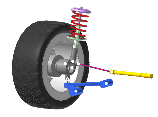
4. Click Open. The model is shown in the following figure.

   

The MacPherson strut is a type of suspension system used in automobiles. It was first developed by Earle S. MacPherson and has a simple structure, making it small, light and inexpensive. It is mainly used in small and mid-sized vehicles. However, it is difficult to predict changes in the camber and toe when the suspension is compressed.

The sample model used in this tutorial measures the changes that occur in the tire when the suspension is compressed. When you apply a vertical force to the tire and move it, the behavior of the tire changes depending on the position and orientation of each component.

11.3.2.3.2. To check the components in the model:

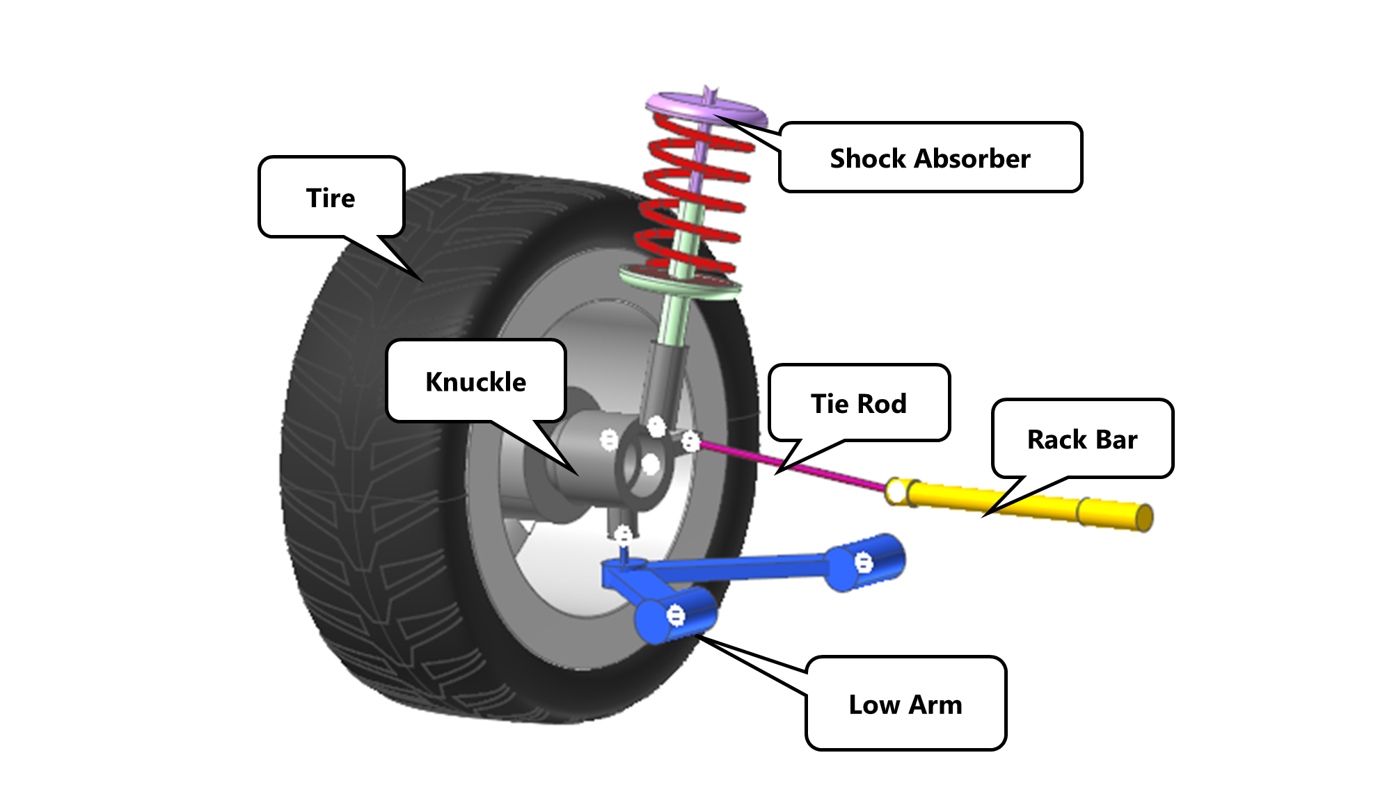
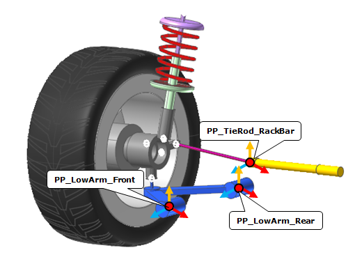
This model consists of a tire, suspension components (knuckle, low arm, and shock absorber), and steering components (tie rod and rack bar).

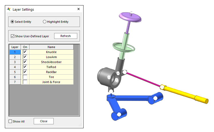
1. In the Render Toolbar, click the Layer Settings tool.

   The dialog window includes a total of 7 layers. Layers 1 to 6 indicate each components of the suspension system, and layer 7 indicates the joint and force.

2. In the Layer Settings dialog window, select the On checkboxes for layers 1 through 7 to confirm the configuration of the model.

11.3.2.3.3. To save the model:

• In the File menu, click the Save As function.

  (You cannot perform the simulation if the model is in the tutorial folder, so you must save the model in a different folder.)

11.3.2.3.4. To perform parametric modeling:

This sample model uses Parametric Points (PPs) and Parametric Values (PVs) for modeling. If you change a few of the PPs in the model, its geometry as well as its joints and forces change according to the changes in the points, forming a model with new dynamic properties.

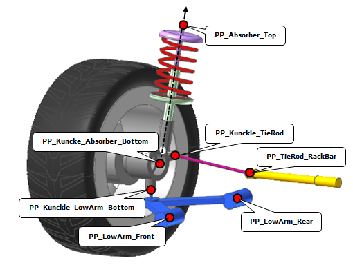
If you change a few of the PPs in the model, the geometry as well as joints and forces connected to those PPs also change.

PP Name	Modified Body	Modified Joint / Force
PP_Absorber_Top	ShockAbsorber, Knuckle	TraJoint_Knuckle_ShockAbsorber Bushing_Ground_ShockAbsorber Spring_Knuckle_ShockAbsorber
PP_Knuckle_Absorber_Bottom	ShockAbsorber, Knuckle	TraJoint_Knuckle_ShockAbsorber Spring_Knuckle_ShockAbsorber
PP_Knuckle_LowArm_Bottom	Knuckle, Low Arm	Spherical_Knuckle_LowArm
PP_LowArm_Front	Low Arm(Front)	Bushing_Ground_LowArm_Front
PP_LowArm_Rear	Low Arm(Rear)	Bushing_Ground_LowArm_Rear
PP_Knuckle_TieRod	Knuckle, TieRod	Spherical_Knuckle_TieRod
PP_TieRod_RackBar	TieRod, RackBar	Spherical_RackBar_TieRod Fixed_Ground_RackBar

11.3.2.3.5. To Preform Parametric Value Modeling

Among the PPs defined above, the X, Y, and Z coordinates of the PP_TieRod_RackBar, PP_LowArm_Front, and PP_LowArm_Rear points are defined using PVs to allow you to change them easily.

PV_TieRod_RackBar_X	X coordinate of the PP_TieRod_RackBar point
PV_TieRod_RackBar_Y	Y coordinate of the PP_TieRod_RackBar point
PV_TieRod_RackBar_Z	Z coordinate of the PP_TieRod_RackBar point
PV_LowArm_Front_X	X coordinate of the PP_LowArm_Front point
PV_LowArm_Front_Y	Y coordinate of the PP_LowArm_Front point
PV_LowArm_Front_Z	Z coordinate of the PP_LowArm_Front point
PV_LowArm_Rear_X	X coordinate of the PP_LowArm_Rear point
PV_LowArm_Rear_Y	Y coordinate of the PP_LowArm_Rear point
PV_LowArm_Rear_Z	Z coordinate of the PP_LowArm_Rear point

11.3.2.3.6. To run the simulation:

1. On the Analysis tab, in the Simulation Type group, click the Dynamic / Kinematic Analysis function.

2. Check the results.

   

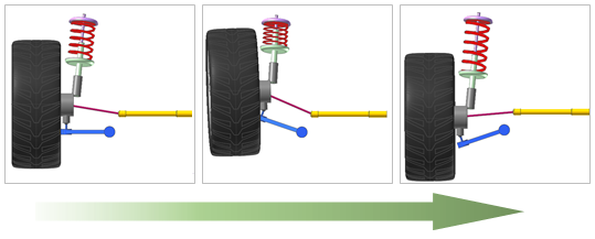
Apply the Z-direction CMotion to the tire to compress and decompress the suspension. You can see that the orientation of the tire changes as it twists from the vertical motion. This twist is due to the structural characteristics of the suspension.

11.3.3. Run Modification Mode

11.3.3.1. Task Objectives

In this chapter, you will learn how to create a template to be used in Modification Mode and run a sample model.

11.3.3.2. Estimated Time to Complete

20 minutes

11.3.3.3. Creating a Modification Template

In this section, you will learn how to create a modification template and control parameters in the RecurDyn model.

11.3.3.3.1. To create a Template_Format sheet:

Define the template to be used in Modification Mode.

1. Open Excel and then create a sheet called Template_Format.

2. In the Template_Format sheet, enter the header and parameter information that defines the template format.

   

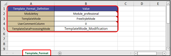
   Template_Format_Definition	Value
   ModuleKey	Module_professional
   TemplateMode	FreeStyleMode
   UserCommentColum	0
   TemplateDataProcessingMode	TemplateMode_Modification

   • ModuleKey: Select a RecurDyn Product module.

   • TemplateMode: Select a Parameter arrangement method.

   • UserCommentColumn: Enter a value between 1and 5 to use one of the columns between A and E in the sheet. If you don’t want to use a column, enter 0.

   • TemplateDataProcessingMode: From Creation Mode, Modification Mode, or Creation and Modification Mode, Select a Template Mode.

   Tip

   Copying the header and parameters using the eTemplate Helper

   1. On the Customize tab, in the eTemplate group, click the Helper function to run the eTemplate Helper.

      

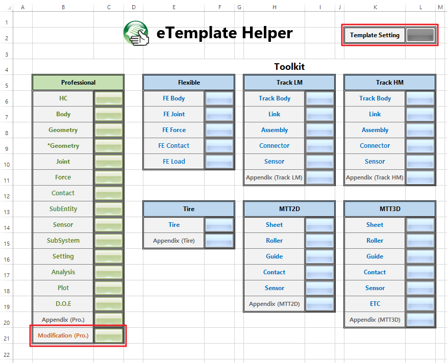
   2. Click the Template Setting button.

   3. Copy the header and parameters of the Template_Format sheet to the template.

   4. Edit the values so that they fit the tutorial.

You may also need to add additional headers and parameters as you continue with this tutorial. You can do so easily by using the Modification (Pro.) sample.

(Note: Generally, the values received in Modification Mode use the header names and parameter names provided in Creation Mode. However, there are some exemptions. For more information about these exemptions, refer to Helper Modification (Pro.).)

Or, you can copy the headers and parameters from the completed template file provided by RecurDyn.

(Template file path: <InstallDir>\Help\Tutorial\eTemplate\Tut3_MacphersonStrut_DesignStudy\Macpherson_Strut_Template.xlsx)

11.3.3.3.2. To create a Template_Data sheet:

You must configure the Template_Data sheet in order to enter the values used in Modification Mode.

1. Create a sheet called Template_Data.

2. In the Template_Data sheet, enter the headers and parameters for Modification Mode.

   

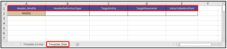
   Header_Modify	HeaderDefinitionType	TargetEntity	TargetParameter	ValueToBeModified
   Modify

For the Modification Mode parameter, enter the following values:

• HeaderDefinitionType: Header name for the target entity

• TargetEntity: Name of the target entity

• TargetParameter: Name of the target parameter

• ValueToBeModified: Value to be modified

11.3.3.3.3. To enter the parameters used to change a PV value:

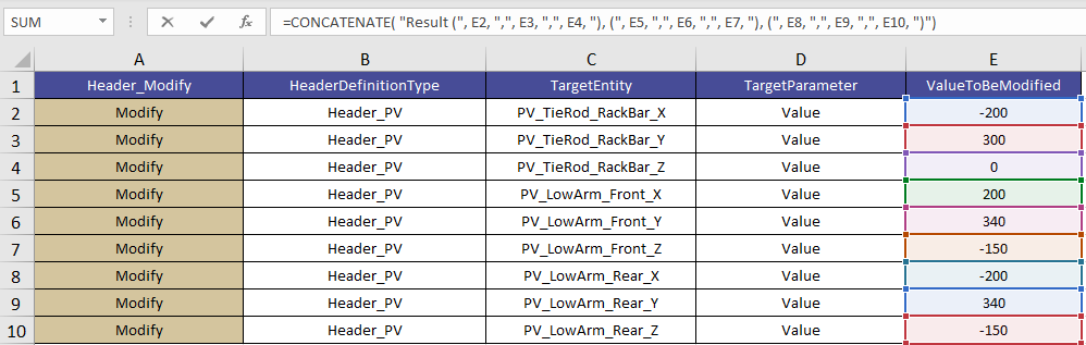
To change a PV value in Modification Mode, you must know the names related to the PV in Creation Mode. Also, you need to know the name of the entity to be modified in the sample model. Enter this information, as shown in the following figure, and then enter the value to be modified.

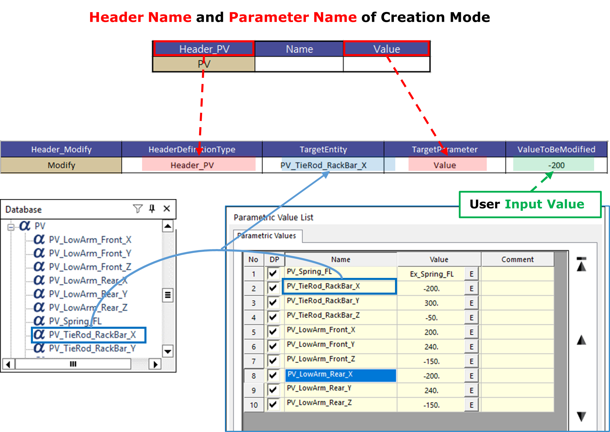
Define the parameters of the PV, as shown in the following figure.

• In ValueToBeModified, enter 0 for PV_TieRod_RackBar_Z, and enter the same values as in the model for others.

  Header_Modify	HeaderDefinitionType	TargetEntity	TargetParameter	ValueToBeModified
  Modify	Header_PV	PV_TieRod_RackBar_X	Value	-200
  Modify	Header_PV	PV_TieRod_RackBar_Y	Value	300
  Modify	Header_PV	PV_TieRod_RackBar_Z	Value	0
  Modify	Header_PV	PV_LowArm_Front_X	Value	200
  Modify	Header_PV	PV_LowArm_Front_Y	Value	240
  Modify	Header_PV	PV_LowArm_Front_Z	Value	-150
  Modify	Header_PV	PV_LowArm_Rear_X	Value	-200
  Modify	Header_PV	PV_LowArm_Rear_Y	Value	240
  Modify	Header_PV	PV_LowArm_Rear_Z	Value	-150

• Save the template file.

11.3.3.4. Running a File in Modification Mode

In this section, you will learn how to open the sample model and run the template in Modification Mode.

11.3.3.4.1. To run the Modification Mode Template

1. On the Customize tab, in the eTemplate group, click the Modify function. The Run Modification Mode dialog window appears.

   

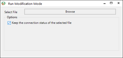
2. Click Browse to open and run the template file created previously.

3. Check the model.

   

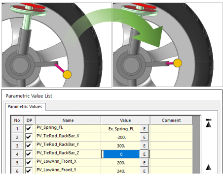
If you open the PV dialog window, you can see that the PV_TieRod_RackBar_Z value has changed from -50 to 0. The model is also modified accordingly.

11.3.4. Run Plot Automation

11.3.4.1. Task Objectives

In this chapter, you will learn how to obtain simulation results automatically using the Plot Automation function of the eTemplate.

11.3.4.2. Estimated Time to Complete

20 minutes

11.3.4.3. Obtaining Results Automatically

In this section, you will learn how to use the Plot Automation function to automate the whole process from modifying the model using Modification Mode to performing the simulation and plotting the results on a graph.

11.3.4.3.1. To enter the simulation parameters:

You must run the simulation immediately after the model is modified. Add the simulation parameters shown in the following figure to the Template_Data sheet in order to run the simulation automatically after the Modification Mode operation is finished.

1. Save Model: Save the model before running the simulation.

   Header_Process_Save	FileName
   Process_Save	Macpherson_Strut

2. Run Simulation: Perform a dynamic analysis.

   Header_Process_Analysis	SimulationRun	AnalysisMode
   Process_Analysis	TRUE	Dynamic

3. Remove Message dialog window: Remove the message dialog window that appears when the Modification Mode operation or the simulation finishes.

   Header_Setting_eTemplate	UseShowImportSuccessMessage	UseShowAnalysisSuccessMessage
   Setting_eTemplate	FALSE	FALSE

11.3.4.3.2. To enter the plot automation parameters:

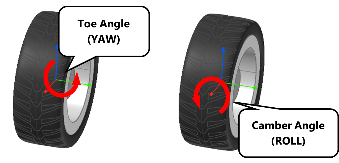
You can get the Toe Angle and Camber Angle using the Yaw and Roll values of the tire. Define the curve that represents the Z axis position of the tire as shown in the following figure.

• Toe Angle Curve

  • X axis: Bodies/Tire/Pos_TZ

  • Y axis: Bodies/Tire/Pos_YAW

• Camber Angle Curve

  • X axis: Bodies/Tire/Pos_TZ

  • Y axis: Bodies/Tire/Pos_Roll

Add the Plot Automation parameters to the Template_Data sheet.

1. Define the curve data: Define the X axis and Y axis data of the curve to be drawn.

   Header_Info_Plot_CurveData	Name	XData	YData	RPLTFileIdentifier	Legend
   Info_Plot_CurveData	CurveData_ToeAng	Macpherson_Strut/Bodies/Tire/Pos_TZ	Macpherson_Strut/Bodies/Tire/Pos_YAW	RecentRPLTFile	ToeAngle
   Info_Plot_CurveData	CurveData_CamberAng	Macpherson_Strut/Bodies/Tire/Pos_TZ	Macpherson_Strut/Bodies/Tire/Pos_ROLL	RecentRPLTFile	CamberAngle

   • XData: The X axis data of the curve

   • YData: The Y axis data of the curve

   • RPLTFileIdentifier: The information of RPLT file to get the curve. If you want to use the RPLT file of current simulation, input the “RecentRPLTFile”

   • Legend: The legend name of the curve

   Tip

   Dragging and dropping the XData and YData input data

   Drag and drop the relevant data from the Plot Database Window to the input field in the Excel sheet to copy the data path.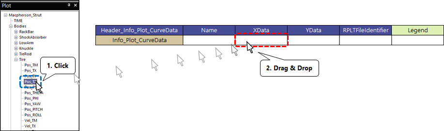

   

2. Define axes: Define the X axis and Y axis format of the curve.

   Header_Info_Plot_XAxis	Name	Title	Max	Min	Decimals	MajorTickStep
   Info_Plot_XAxis	XAxis_PosZ	ZPosition (mm)	100	-100	0	20

   Header_Info_Plot_YAxis	Name	Title	Max	Min	MajorTickStep	AxisPositionType
   Info_Plot_Yaxis	YAxis_ToeAng	ToeAng (deg)	8	-8	2	Left
   Info_Plot_Yaxis	YAxis_CamberAng	CamberAngle (deg)	3	-1	0.5	Left

   • Title: The string displayed on the axis

   • Max/Min: The minimum and maximum values of the axis

   • Decimals(Info_Plot_Xaxis): The number of decimal places shown in the values on the X axis

   • MajorTickStep: The difference in values between adjacent markings on the axis

   • AxisPositionType(Info_Plot_Yaxis): The position of the Y axis

3. Define the curve to be drawn on the plot: Use the data defined in the steps 1 and 2 to define the graph to be drawn on the plot.

   Header_Process_Plot	UseDrawPlot	TargetPage	TargetPane	TargetCurveData	XAxisProperty	YAxisProperty
   Process_Plot	TRUE	1	1	CurveData_ToeAng	XAxis_PosZ	YAxis_ToeAng
   Process_Plot	TRUE	1	2	CurveData_CamberAng	XAxis_PosZ	YAxis_CamberAng

   • UseDrawPlot: Draw Flag

   • TargetPage: The page on which the curve data is drawn

   • TargetPane: The pane on which the curve data is drawn

   • TargetCurveData: The curve data information

   • XAxisProperty: The X axis format of the curve

   • YAxisProperty: The Y axis format of the curve

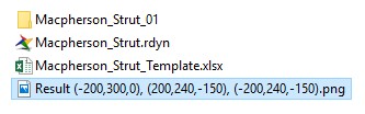
4. Export as an image: Export the curve drawn on the plot as an image file. If you don’t specify a separate folder path, the image file is saved in the same folder as the template file.

   Header_Plot_Export_Image	FileName
   Plot_Export_Image	Result (-200,300,0), (200,240,-150), (-200,240,-150)

   Use the CONCATENATE function of Excel to include the X, Y, and Z coordinates of the PP_TieRod_RackBa, PP_LowArm_Front, and PP_LowArm_Rear points in the name of the image file.

   = CONCATENATE( “Result (”, E2, “,”, E3, “,”, E4, “), (”, E5, “,”, E6, “,”, E7, “), (”, E8, “,”, E9, “,”, E10, “)”)

   

11.3.4.4. Using the Automation Tool

In this section, you will learn how to use the MacPherson Strut model provided in this tutorial and the template you created to examine the dynamic properties of the suspension system

11.3.4.4.1. To run the Modification Mode template:

1. Open the sample model in RecurDyn.

2. On the Customize tab, in the eTemplate group, click the Modify function.

   The Run Modification Mode dialog window appears.

3. Click Browse to locate and run the template file created previously.

   

The model is modified automatically, and the simulation is performed. Once the simulation is finished, the plot data is drawn automatically, and the curve is saved as an image file in the same path as the template file.

The section in which the Tire_Pos_Z value is positive indicates when the suspension is being compressed. If you look at the behavior of the tire in the section, you can see that both the Toe Angle (Yaw) and Camber Angle (Roll) tend to increase. That is, the suspension shows tendencies towards Toe In and a Positive Camber Angle.

Toe In helps increase the stability of the vehicle when driving straight and is used in normal vehicles. In contrast to this, a Positive Camber Angle can reduce the performance of a vehicle and damage its suspension, so it is not used in normal vehicles.

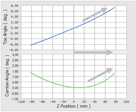
Let’s change the model so that the Positive Camber Angle becomes a Negative Camber Angle.

11.3.4.4.2. To modify the model and run the simulation:

Let’s modify the PV values so that the suspension model includes both Toe In and Negative Camber tendencies.

1. In the template file, change the ValueToBeModified value of PV_LowArm_Front_Y and PV_LowArm_Rear_Y to 340.

   Header_Modify	HeaderDefinitionType	TargetEntity	TargetParameter	ValueToBoModified
   Modify	Header_PV	PV_TieRod_RackBar_X	Value	-200
   Modify	Header_PV	PV_TieRod_RackBar_Y	Value	300
   Modify	Header_PV	PV_TieRod_RackBar_Z	Value	0
   Modify	Header_PV	PV_LowArm_Front_X	Value	200
   Modify	Header_PV	PV_LowArm_Front_Y	Value	340
   Modify	Header_PV	PV_LowArm_Front_Z	Value	-150
   Modify	Header_PV	PV_LowArm_Rear_X	Value	-200
   Modify	Header_PV	PV_LowArm_Rear_Y	Value	340
   Modify	Header_PV	PV_LowArm_Rear_Z	Value	-150

2. Save the template file.

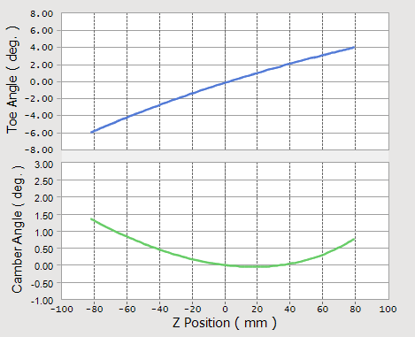
3. Return to the sample model. Then, on the Customize tab, in the eTemplate group, click the Modify function.

   Since the template file is already linked to the sample model, the model is modified immediately, and the plot is drawn without any additional input.

   Even after the modification, the suspension still shows a tendency towards a Positive Camber Angle.
   

   Let’s modify the Z axis of the LowArm and run the simulation again.

4. In the template file, change the ValueToBeModified value of PV_LowArm_Front_Z and PV_LowArm_Rear_Z to -100

5. Save the template file.

6. Return to the sample model. Then, on the Customize tab, in the eTemplate group, click the Modify function.

   The model is modified, and the plot is drawn.

   Header_Modify	HeaderDefinitionType	TargetEntity	TargetParameter	ValueToBoModified
   Modify	Header_PV	PV_TieRod_RackBar_X	Value	-200
   Modify	Header_PV	PV_TieRod_RackBar_Y	Value	300
   Modify	Header_PV	PV_TieRod_RackBar_Z	Value	0
   Modify	Header_PV	PV_LowArm_Front_X	Value	200
   Modify	Header_PV	PV_LowArm_Front_Y	Value	340
   Modify	Header_PV	PV_LowArm_Front_Z	Value	-100
   Modify	Header_PV	PV_LowArm_Rear_X	Value	-200
   Modify	Header_PV	PV_LowArm_Rear_Y	Value	340
   Modify	Header_PV	PV_LowArm_Rear_Z	Value	-100

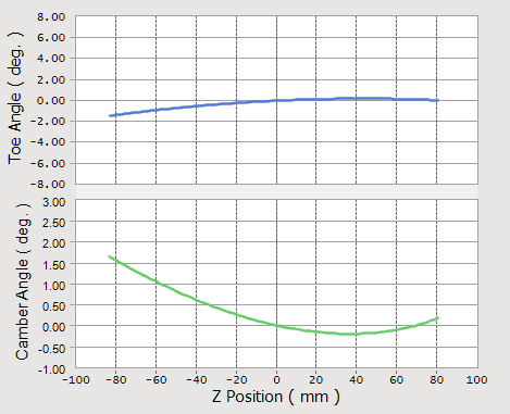
   The model shows a tendency towards a Negative Camber Angle, but the Toe Angle has decreased significantly and now shows a tendency towards Toe Out

   

   Let’s modify the Z axis of the TireRod and run the simulation again to be Toe In.

7. In the template file, change the ValueToBeModified value of PV_TieRod_RackBar_Z to 50.

8. Save the template file.

9. Return to the sample model. Then, on the Customize tab, in the eTemplate group, click the Modify function.

   The model is modified, and the plot is drawn.

   Header_Modify	HeaderDefinitionType	TargetEntity	TargetParameter	ValueToBoModified
   Modify	Header_PV	PV_TieRod_RackBar_X	Value	-200
   Modify	Header_PV	PV_TieRod_RackBar_Y	Value	300
   Modify	Header_PV	PV_TieRod_RackBar_Z	Value	50
   Modify	Header_PV	PV_LowArm_Front_X	Value	200
   Modify	Header_PV	PV_LowArm_Front_Y	Value	340
   Modify	Header_PV	PV_LowArm_Front_Z	Value	-100
   Modify	Header_PV	PV_LowArm_Rear_X	Value	-200
   Modify	Header_PV	PV_LowArm_Rear_Y	Value	340
   Modify	Header_PV	PV_LowArm_Rear_Z	Value	-100

   The model shows both the Negative Camber Angle and Toe In tendencies.

   

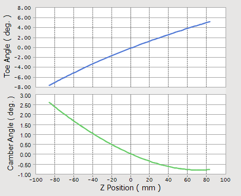
All the result graphs produced in the test are automatically saved as image files in the same folder as the template file. You can use the image files later to report the results.