3.3. Paper Distributing System Tutorial (AutoDesign)

3.3.1. Outline of Tutorial Sample C

Model

Description

Sample_C

Paper Distributing System Design Problem: This design is a robust design and a 6-sigma design problem. Especially, 3 variables are noise factors and 2 variables are random design variables. Unlike Taguchi approach or other design tools, AutoDesign helps the designers to define a robust design formulation and 6-sigma constraints easily. Also, this problem results show how AutoDesign is efficient to solve a robust design and a 6-sigma constraint problem. Key Point: Study the conceptual differences between a robust design and 6-sigma design. Also, understand how AutoDesign defines the noise factors and random design variables.

3.3.2. Paper Distributing System Problem

Robust Design Optimization differs from the deterministic design optimization you just performed in Sample-A and Sample-B, in that it takes into account the variability of the components which make up the system being optimized. For example, if temperature fluctuation or manufacturing conditions caused variability in the front link angle, you could measure this variability and input the standard deviation into the robust design optimization. The optimization would then give results which would tell you the variability of the system performance, and therefore aid in the design of a system robust to the variation of its individual components.

RecurDyn/AutoDesign allows you to define the sigma level to which you want to optimize. That is, you can define the “percent feasible”, or the fraction of the produced systems which will satisfy the quality constraints. A common standard is to design to 6-sigma, which means that 99.9999998% of the produced systems will satisfy the quality constraints. For more information on robust design optimization and design for 6-sigma (DFSS), refer to the RecurDyn Theoretical and Guideline Manual.

Open files related in Sample-C
Sample		<InstallDir>\Help\Tutorial\AutoDesign\PaperDistributingSystem\Example\Sample_C1.rdyn
Solution	1	<InstallDir>\Help\Tutorial\AutoDesign\PaperDistributingSystem\Solutions\Sample_C1.rdyn
	2	<InstallDir>\Help\Tutorial\AutoDesign\PaperDistributingSystem\Solutions\Sample_C2.rdyn

Note

If you change the file path at discretion, it can be located in any folder that you specify.

3.3.3. Loading the Model and Viewing the Animation

3.3.3.1. To load the base model and view the animation:

1. On your Desktop, double-click the RecurDyn icon. RecurDyn starts and the Start RecurDyn dialog box appears.

2. Close Start RecurDyn dialog box. You will use an existing model. In the Quick Access toolbar, click the Open and select Sample_C1.rdyn from the same directory where this tutorial is located. The MTT2D appears in the modeling window.

3. Double-click the model on the screen to enter MTT2D toolkit. Then, Model name is changed from Model1 into MTT2D@Model1 on the left upper part in screen.

4. Click Dynamic/Kinematic.

5. Click Simulate.

6. In order to view result, click Play.

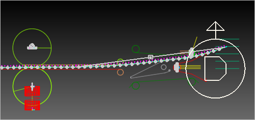
The sheet runs through the upper and lower baffles and reaches to the second tray.

3.3.4. Design Variables

Design variables will be the factors of the model which you can control. Figure 3.46 and Figure 3.47 are the window and the diagram showing these factors on the model.

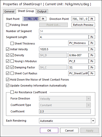
Figure 3.46 Three design variables for random constants

In the SheetGroup1 dialog, the thickness, young’s modulus and curl radius are selected as DV1 ~ DV3. These variables are un-controllable factors from the viewpoint of mechanism designers. Thus, we consider them as random constants.

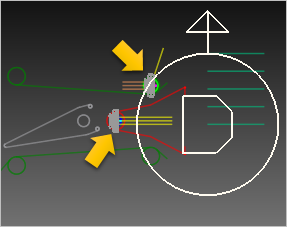
Figure 3.47 Two design variables with tolerances

In Figure 3.47, the vertical locations of two guides are selected as design variables. In MTT2D, the guide positions cannot be defined by using parametric values. Thus, they are not design variables directly. To overcome this situation, we introduce the motion that can include the parametric values. Two motions use the following expressions, respectively.

• PV_Yupper*STEP(TIME, 0, 0, 0.01, 1)

• PV_Ylower*STEP(TIME, 0, 0, 0.01, 1)

3.3.4.1. Defining the Design Variables

3.3.4.1.1. To create a design parameter:

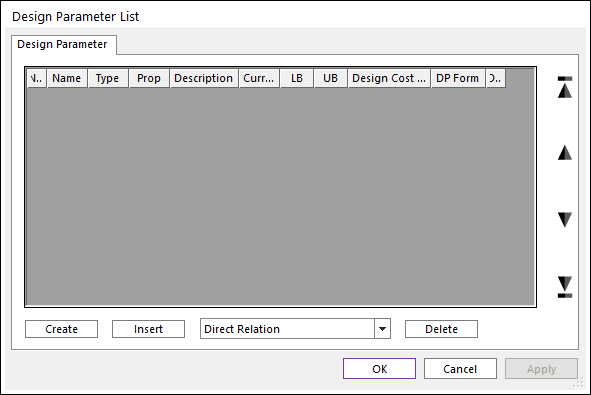
1. From the AutoDesign menu, click Design Parameter. This will bring up the Design Parameter List dialog shown below.

   

2. Click Create to create a new design parameter. In the Direct Relation dialog that appears, change the name from DP1 to DP_SheetCurlFactor.

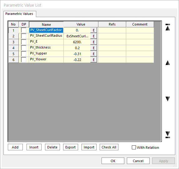
3. Press PV to bring up the Parametric Value List dialog. Select the PV_SheetCurlFactor parametric value by clicking on its name. When selected, it should be highlighted in blue, as shown at below.

   

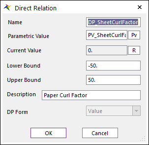
4. Click OK to choose this as the design parameter. Back in the Direct Relation dialog, define upper and lower bounds (-50, 50). Enter a description (Paper Curl Factor) in the Description field. When completed, the dialog should appear as shown at below.

   

5. Press OK to return to the Design Parameter List dialog box.

6. Create design parameter for spring mount height, similarly, using the following settings:

   Name	Parametric Value	Lower Bound	Upper Bound	Description
   DP_Modulus	PV_E	5200	7200	Paper_Modulus_E
   DP_Thickness	PV_thickness	0.1	0.3	Paper_Thickness
   DP_UpperPos	PV_Yupper	-1	1	Upper baffle Y loc
   DP_LowerPos	PV_Ylower	-1	1	Lower baffle Y loc

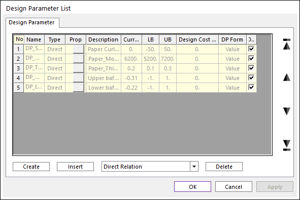
7. Return to the Design Parameter List dialog and check the checkboxes under the DV column for both of the design parameter you just created. This activates both as Design Variables, which will be used in the Design Study and Design Optimizations to follow. When completed, the Design Parameter List dialog should appear as shown at below.

   

   Note

   To go back and edit a design parameter, click the button under the Prop. column.

8. Press OK to close the Design Parameter List dialog box.

3.3.5. Defining the Performance Indexes

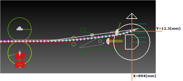
Let’s consider the paper distributing system as shown below The goal of the mechanism is to design the baffler y-positions for the paper to pass through the target position nevertheless the material property (Young’s modulus, thickness and curl radius etc.) variations of the paper. In this problem, the material property variations are called as noise factors and the baffler positions are done as design variables. If the design variables have +/- tolerances, we call them as random design variables. In AutoDesign, the noise factors are called as random constants.

3.3.5.1. To create an analysis response:

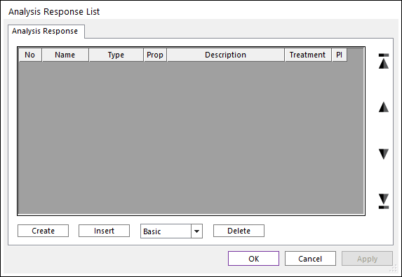
1. From the AutoDesign menu, click Analysis Response. This will bring up the Design Response List dialog as shown below.

   

2. Click Create to create a new analysis response. In the Analysis Response - Basic dialog that appears, change the name from AR1 to AR_Ysensor1.

   

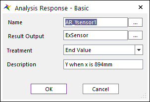
3. Press EL to bring up the Expression List dialog. Select the ExSensor expression by clicking on its name. When selected, it should be highlighted in blue, as shown below.

   

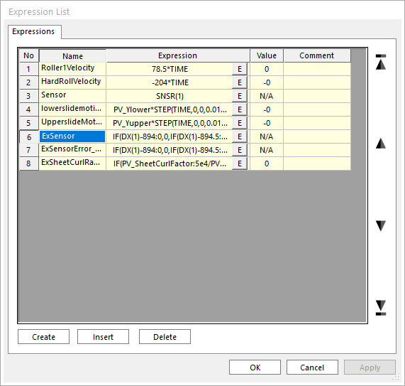
4. Click OK to choose this as the expression to use.

5. Back in the Analysis Response - Basic dialog, for the Treatment, select End Value from the dropdown list. Enter a description (Y where x is 894mm) in the Description field. When completed, the dialog should appear as shown above.

6. Press OK.

   Note

   To go back and edit an analysis response, click the button under the Prop. column

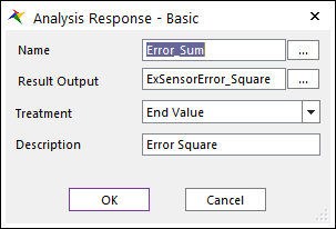
7. Create one more analysis response using the following values:

   • Name: Error_Sum

   • Expression Name: ExSensorError_Square

   • Treatment: End Value

   • Description: Error Square

   

   The treatment parameter is used to control how you extract a single numerical value from a curve which varies over time. For example, setting the treatment to End Value will assign the value of the curve at the end of simulation, while Min Value will assign the lowest value that the curve reaches during the simulation.

8. Return to the Analysis Response List window and check the checkbox under the PI column corresponding to the analysis responses you just created. This activates them as Performance Indexes, which will be used in the Design Study and Design Optimizations to follow. When completed, the Analysis Response List window should appear as shown below.

   

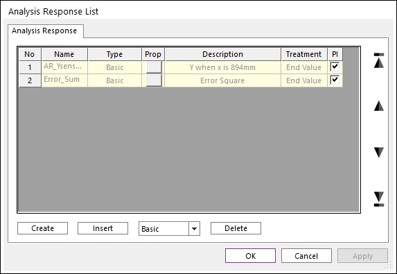
9. Press OK to close the Analysis Response List dialog.

10. Save the model.

3.3.6. Running a Robust Design Optimization

We will now run an optimization in which the objective is to minimize the variance of position error, and constraints are set on the y-position error.

The random design variables and random constants are listed in Table 3.2.

Table 3.2 List of random design variables and constants

Description	Current Values	Deviations	Remark
Upper baffle position	-0.31	-/+ 0.05	Random Design Variable
Lower baffle position	-0.22	-/+ 0.05	Random Design Variable

The robust design optimization problem is defined as:

Minimize Variance

Subject to

The paper position at x=894 (mm) = Target position

and

-1.0 =< Upper baffle position -/+ deviation =< 1.0 -1.0 =< Lower baffle position -/+ deviation =< 1.0.

The value of variance is affected from the tolerance of design variables and the deviations of noise factors. Thus, the robust design optimization problem is to find the design variables to minimize the variation of position errors, which is a typical example of robust design optimization.

3.3.6.1. To run a robust design optimization:

1. From the AutoDesign menu, select DFSS/Robust Design Optimization. The Design Variable dialog should appear as shown below. You should define the red-box parts.

   

   Unlike the design optimization, three selections are newly shown. They are Statistical Info, Dev. Type and Dev. Value. The detail descriptions of them are explained in Guideline manual. In the Statistical info, you can define which variables are random or deterministic. If the variable has tolerance or deviation, then it is random. Otherwise, it is a deterministic variable. In the Dev. Type, you can define that the deviation of variable is an absolute magnitude or the ratio of design value. SD denotes the absolute magnitude. COV does the relative ratio. Paper properties are defined as random constant because they are only noise factors.

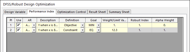
2. Click the Performance Index page.

3. Change the objective function according to the table below.

   AR	Definition	Goal	Weight/Limit Value	Robust Index	Alpha Weight
   AR_Ysensor1	Constraint	EQ	12.3	NA	NA
   AR_Ysensor1	Objective	MIN	1	1	0

   It is noted that AR2 is not used in Sample_C1.

   After making the changes, the dialog should appear as shown below. The grey part represents the deactivated values.

   

   In DFSS/Robust design optimization, the design objective is internally represented as:

   PI = Weight*(AR*Alpha_Weight+Sigma*Robust_Index)

   The value of Weight represents the relative importance of the selected AR in the multiple objectives. Alpha_Weight and Robust_Index are the flags of two responses. These values should be 0 or 1. 0 represents that the corresponding response is neglected.

   If Alpha_Weight=1 and Robust_Index=0, then minimize Weight*AR.

   If Alpha_Weight=0 and Robust_Index=0, then minimize Weight*Sigma.

   If Alpha_Weight=0 and Robust_Index=1, then minimize Weight*(AR+Sigma).

   If both values are 0, then make no design formulation. It is a logical error.

4. Click on the Optimization Control page.

5. Change the settings so that they appear as shown below.

   

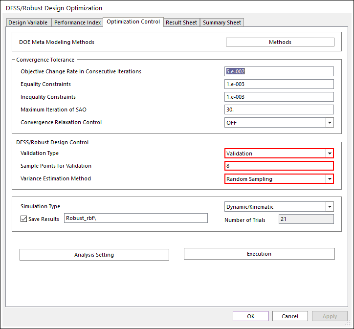
6. For the convergence tolerance, the default values are used. Unlike the design optimization module, DFSS/Robust Design Control is newly shown. In the above figure, the red color box shows the DFSS/Robust Design control. The detail information of them is explained in Guideline Manual. As you can see, AutoDesign solves the robust design problem by using the meta-models.

   Although the analysis responses are validated when the meta-model is updated during optimization process, the standard deviation is estimated from meta-models. Thus, the variance values of final design are not validated. In the Validation Type, there are three types such as None, Validation and Validation & Re-Optimization. When Validation is selected, AutoDesign performs the exact analyses for the sampled points within the deviation ranges at the final design. Then, estimate the sample variance. In the Variance Estimation Method, there are two types such as Taylor Series method and Random Sampling method, which are the variance approximation method from meta-models, which are explained in Guideline manual.

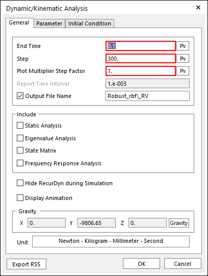
7. Check the analysis setting by clicking Analysis Setting. As explained in Sample-A and Sample-B, it is noted that the accuracy of analysis responses depends on the number of STEP.

   

8. Click Execution to run the optimization with the settings you just made. Then, you can see the summary of the optimization formulation shown at below. Then, click OK. The optimization will be progressed.

   

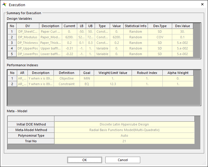
9. To view the result of the design optimization after optimization is completed, click the Result Sheet page.

   

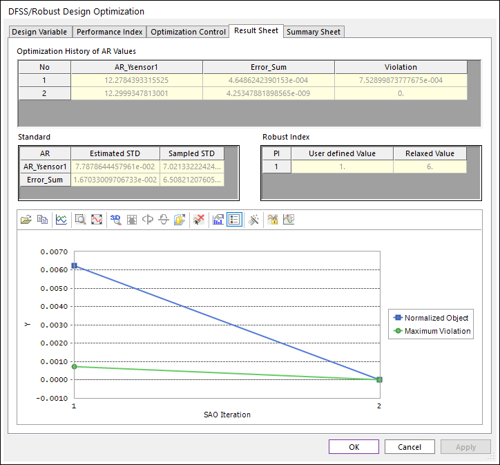
   The optimization process is converged at the 2th iteration. The final design gives that AR1 is 12.29 and its’ approximate Sigma is 0.07 and the sample Sigma is obtained as 0.07. The error between the approximate Sigma and the sample Sigma is caused from the accuracy of meta-models. When the sample Sigma is greater than the estimated ones, you may re-optimize by using Get from Simulation History.

10. Now, check the analysis results in Summary Sheet. When constructing the meta-models, the values of design variables and constants are sampled within their bounds and deviations. If you define the parameter as constant, however, they are not changed during optimization process.

    In the list of design variables, DV4 and DV5 are changed from (-0.31, -0.22) to (-0.34, –0.21 because they are design variables.

    In the list of analysis responses, the optimum values are the analysis responses for the optimum design values and the sample STD (standard deviations) values are evaluated from the sample points for validation. See the optimization control menu at the above Step 7.

    

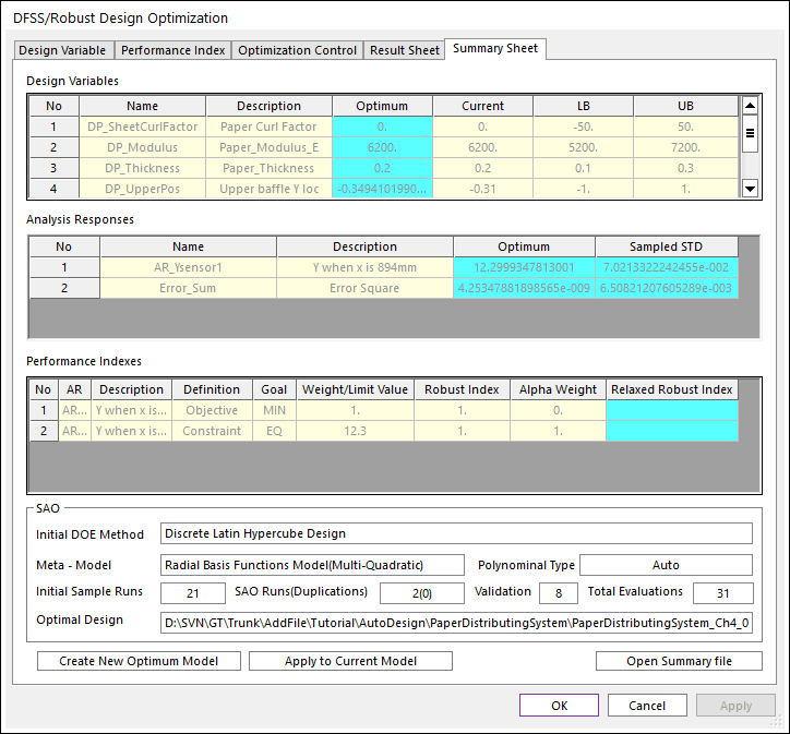
    In the SAO summary, the total number of evaluations is 31 that include the 21 evaluations for the initial sampling.

11. Save the model. In order to study 6-Sigma design, save as the model as Sample_C2.

3.3.7. Running a 6-Sigma Design Optimization

Load the model Sample_C2.rdyn. As you can see, 6-Sigma design uses the same design variables and analysis responses as Sample_C1. Only the design formulation is different from the robust design. Figure 3.48 shows the design variables, which is the same as Sample_C1.

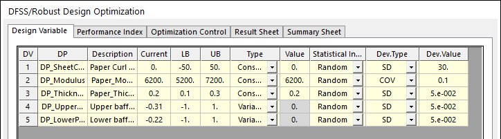
Figure 3.48 The design variables for 6-Sigma Design Optimization

3.3.7.1. To run a robust design optimization:

1. Let’s consider the 6-sigma design optimization formulation, shown in Figure 3.49. The design goal is to minimize the sum of error, which represents (Y_position - 12.3)**2. From the viewpoint of 6-sigma design, the Y_position should satisfy the following inequality relations.

   9.3 =< Y_position -/+ 6*Sigma =< 15.3

   AutoDesign describes the above relation by using two inequality constraints.

   9.3 =< Y_position - 6*Sigma

   Y_position + 6*Sigma =< 15.3

   The signs of - and + positioned before sigma are automatically defined for the inequality constraint types such as GE or LE. Hence, you can define those two inequality constraints shown in Figure 3.49. The grey colored parts are deactivated.

   As explained in Sample_C1, DFSS/Robust design module defines the design objective as

   PI = Weight*(AR*Alpha_Weight+Sigma*Robust_Index)

   For this problem, we want to minimize only AR2. Thus, we define the robust index = 0 and the alpha weight = 1.

   

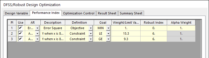
   Figure 3.49 Design optimization formulation for 6-sigma constraints

2. Click the Optimization Control DOE Meta Modeling Methods

3. In order to save the computational time, we will use the analysis results from Sample_C1. Uncheck Select DOE method and Check Get From Simulation History. Then, the Get From Simulation History button will be activated. Click Get From Simulation History.

   

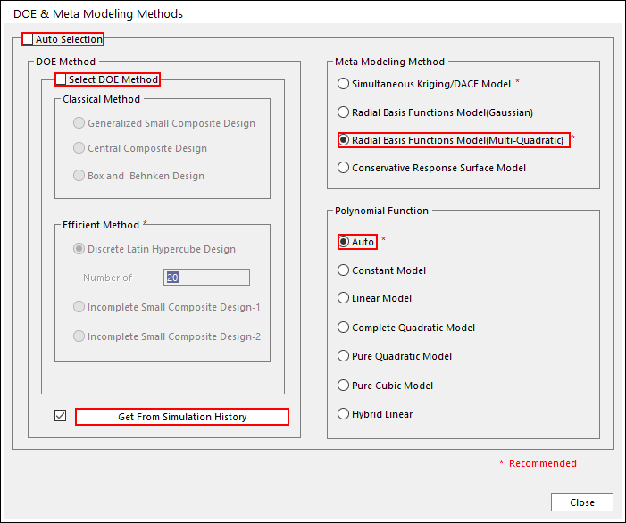
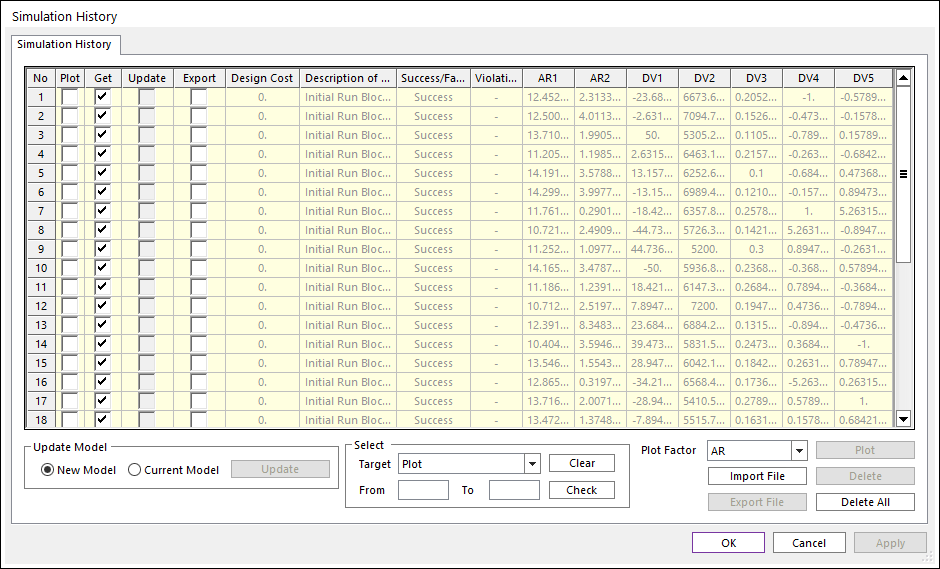
4. Then, you can see the simulation history as below. Then, check the runs in the Get column. In order to compare 6-sigma design optimization with the robust design result, select only the results of Initial Runs for Meta Model. Finally, click OK.

   

5. Now, you will back to the window of DOE Meta Modeling Methods. Then, select Radial Basis Function Model(Multi-Quadratics) for meta-model and Auto for polynomial type.

6. To Return the Optimization Control page, click Close. We will the same convergence tolerances and the same validation information. Thus, click Execution . If all information is the same as Figure 3.50, then push OK.

   

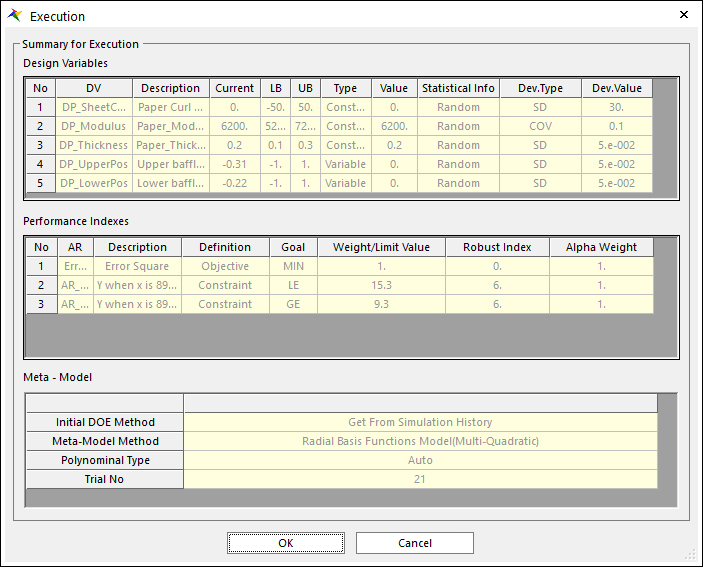
   Figure 3.50 Summary of 6-Sigma design optimization formulation

7. When the optimization process is converged, click the Result Sheet page. Then, the optimization results are shown in Figure Figure 3.51. The final design gives that AR1=11.8 and the estimate Sigma and the sample Sigma are 0.034 and 0.055, respectively. In the robust index check, the relation of AR1+/-6*0.055 satisfies the limit values of 9.3 and 15.3. Thus, the relaxed values for robust indexes are obtained as 6. For more information of 6-sigma design, refer to the Guideline Manual.

   

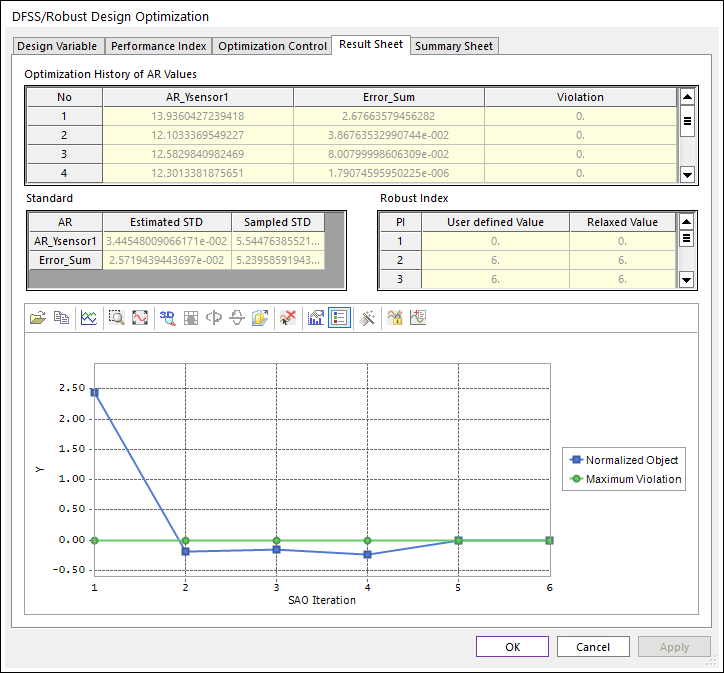
   Figure 3.51 Convergence history of 6-Sigma design optimization

Now, compare the optimization results of Sample_C1 and Sample_C2. Both designs have different design variables (DV4 & DV5) but give nearly equal values of the sample-Sigma. Thus, you can select one of them. For these comparisons, we think that the design result of robust design is better than that of 6-sigma design, because it gives better position of paper at the target position even though their sample variances are nearly equal.