8.3. FFlex Mesher Suspension Tutorial (Durability)
8.3.1. Introduction
Fatigue and durability analyses are designed to determine how long a flexible body or specific area of a flexible body modeled in RecurDyn can stably endure various dynamic loads. Such analyses can also determine how stable a body is. The focus on time distinguishes these forms of analysis from other analysis methods, such as those used to determine maximum stress and maximum deformation rates.
This tutorial teaches you how to use RecurDyn/Durability to determine the fatigue life and fatigue damage in a dynamic system composed of flexible bodies. This tutorial also briefly describes functions and theoretical backgrounds used in RecurDyn/Durability. Thus, even users who do not have a thorough grounding in the theoretical background of durability analysis can learn to use RecurDyn/Durability simply by completing this tutorial.
This tutorial uses the MBD model, which features a simplified system intended for experimental purposes. By following the steps in this tutorial, you will learn how to replace specific sections of the flexible bodies in the model using RecurDyn/Mesher and verify the properties and durability results of these flexible bodies. Later in this tutorial, you will learn how to produce durability results for a specific section of the model.
8.3.1.1. Task Objectives
This tutorial covers the following:
Creating a flexible body using RecurDyn/Mesher
Requirements for durability analysis
Methods of conducting durability analysis
Obtaining durability analysis results
Analyzing durability analysis results
8.3.1.2. Requirements
This tutorial is intended for intermediate users who have read and understood the basic tutorial as well as the FFlex and RFlex tutorials available from RecurDyn. If you have not completed these tutorials, then you are advised to complete them before proceeding with this tutorial. In addition, this tutorial requires a basic understanding of dynamics and the finite element method.
8.3.1.3. Procedures
This tutorial consists of the tasks outlined in the following table. This table also shows the time required to complete each task.
Procedures |
Time (minutes) |
Calling an Rdyn model |
10 |
Creating an FFlex body using Mesher |
15 |
Replacing an RFlex body |
20 |
Creating a patch set to verify the fatigue results |
5 |
Setting fatigue preferences |
5 |
Performing a fatigue evaluation |
5 |
Verifying the fatigue results |
5 |
Total |
65 |
8.3.1.4. Estimated Time to Complete
This tutorial takes approximately 65 minutes to complete.
8.3.2. Calling the Initial Model
8.3.2.1. Task Objective
This chapter teaches you how to open an initial model, simulate it, and observe the behavior of the suspension model.
8.3.2.2. Estimated Time to Complete
10 minutes
8.3.2.3. Calling a Rdyn Model
8.3.2.3.1. To open RecurDyn and call the initial model:
On the Desktop, double-click the RecurDyn icon. When the Start RecurDyn dialog window appears, close it.
From the File menu, click Open.
- From the Durability tutorial path, select the RD_Durability_Start.rdyn file.(The file path: <InstallDir>\Help\Tutorial\PostAnalysis\Durability\FFlexMesherSuspension).
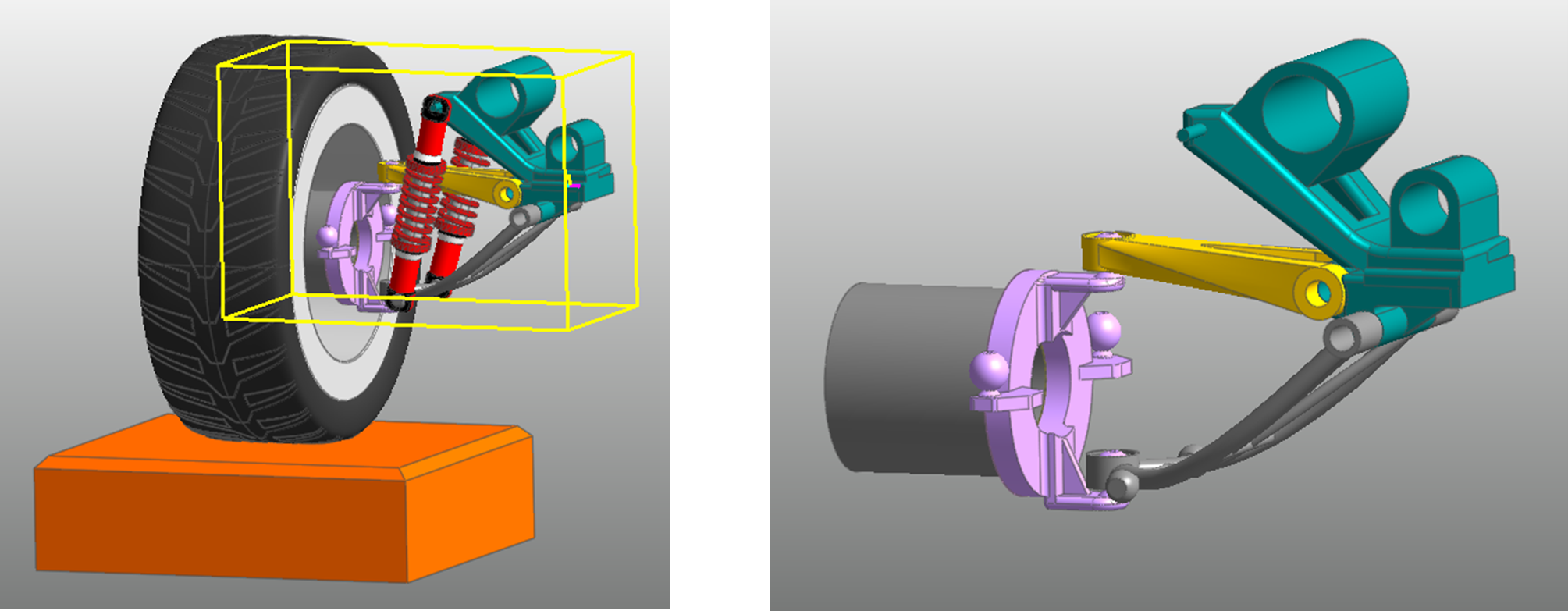
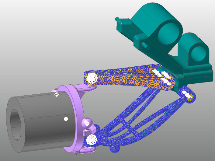
Click Open. The model shown below opens.
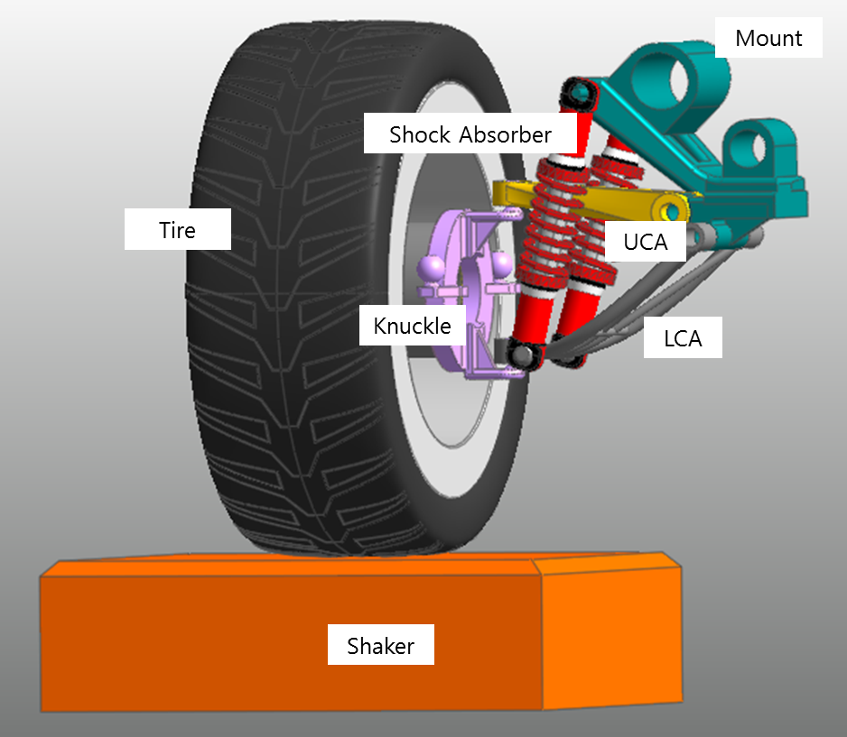
This model is designed to test the durability of the parts in a suspension system. A suspension system absorbs shocks from street surfaces in order to prevent them from being transferred to the vehicle or passengers. In this model, the tire rests on the shaker so that any excitations pass directly from the shaker to the tire and the suspension system.
The suspension system in this model consists of one tire and three subsystems. The three subsystems include two shock absorbers with built-in coil springs and a suspension assembly. The suspension assembly consists of a mount, a knuckle, an LCA (lower connecting arm), and a UCA (upper connecting arm). In this tutorial, you will test the durability of the LCA and the UCA.
8.3.2.3.2. To save the initial model:
From the File menu, click the Save As function.
(Save this model in the different path because it is impossible to simulate directly in the tutorial path.)
8.3.2.4. Running an Initial Simulation with the Suspension Model
In this task, you will run an initial simulation on the model to understand how it operates.
8.3.2.4.1. To run an initial simulation:
From the Simulation Type group in the Analysis tab, click the Dynamic/Kinematic Analysis function. The Dynamic/Kinematic Analysis dialog window appears.
Define the End Time and Step values as follows:
End Time: 1.2
Step: 200
Plot Multiplier Step Factor: 1
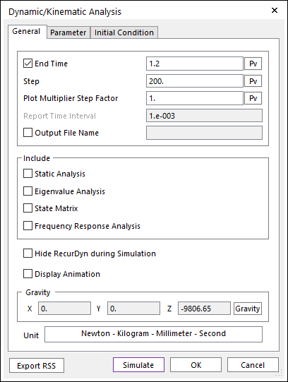
Click Simulate.
8.3.2.5. Viewing the Results
8.3.2.5.1. To view the results:
From the Animation Control group in the Analysis tab, click the Play/Pause function.
The excitation is transferred to the tire through the shaker. The animation shows any possible vibrations or seismic excitation caused by driving the vehicle. At this point, you can observe the behavior of certain devices, including the shock absorbers.
8.3.3. Creating an FFlex Body
This chapter teaches you how to conduct a durability analysis on a flexible body. This procedure maintains some elements of the previous model, such as its joint and force, but replaces certain rigid bodies with flexible bodies to increase the efficiency of the model.
8.3.3.1. Task Objective
This task teaches you how to replace an existing rigid body with a flexible body using the Mesher provided in RecurDyn FFlex (Full Flex).
8.3.3.2. Estimated Time to Complete
15 minutes
8.3.3.3. Creating a UCA Body Mesh
In Assembly mode, double-click the Suspension_Assy created as a Subsystem to enter the Subsystem mode.
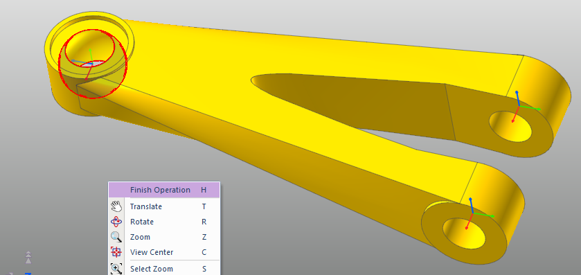
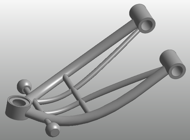
In Subsystem mode, select the UCA body and Right-click the selected body, and select Mesh from the context menu, as shown in the figure to the below.
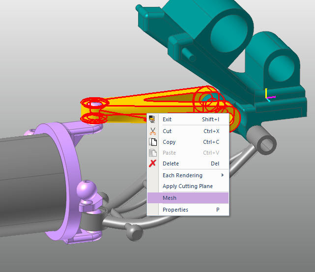
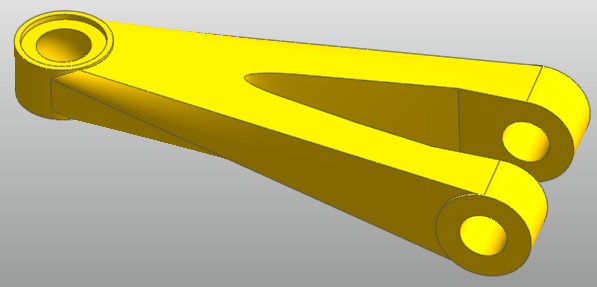
The UCA body appears as shown in the figure below.
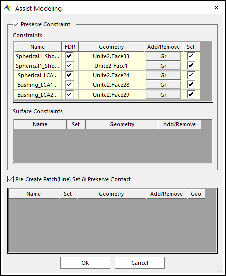
Mesh mode, click the Assist Modeling function from the Mesher group in the Mesher tab. The Assist Modeling dialog window appears.
Tip
The Geometries in the Preserve Constraint are applied to the Assist Modeling dialog automatically when opening the dialog. However, following behind steps are recommended to the user to produce accurate results, especially in the tutorial.
Tip
The FDR checkboxes specify whether or not to create an FDR (Force Distributed Rigid) element after the Mesh operation. The Sel. checkboxes specify whether or not to maintain the joint or force previously created. In this tutorial, these functions are all necessary. Select all of the checkboxes.
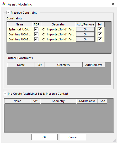
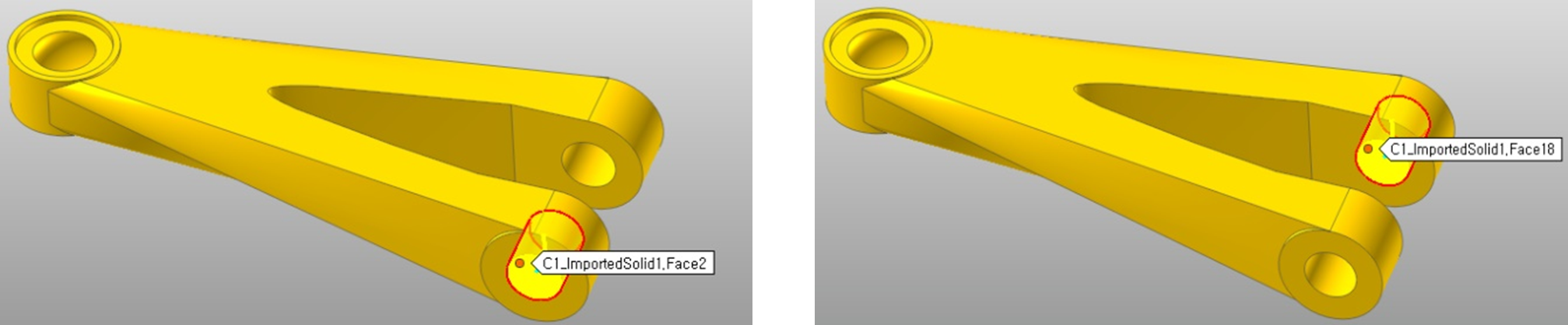
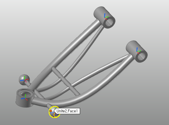
In the Add/Remove column of the dialog window, click Gr to assign the geometries for the areas where the Slave Nodes will be created. Referring to the following page, select the geometries where the slave nodes will be created for the three FDRs. (Tip: When you click the Gr button, a marker appears on the screen indicating where the master node will be generated. This helps you locate the areas to assign slave nodes.)
Tip
Due to the nature of the FDR, the master node is automatically generated at the point where the joint and the force are created. You must define the slave nodes directly.
After all the geometries are assigned, right-click the model, and click Finish Operation.
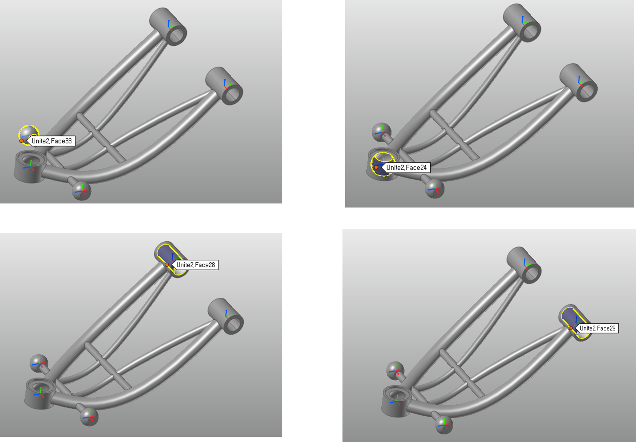
For the other two areas, select the Surfaces where the Slave Nodes will be generated, as shown in figures below.
Once you have selected all the geometry items, click OK.
From the Mesher group in the Mesher tab, click the Advanced Mesh function. The Advanced Mesh dialog window appears.
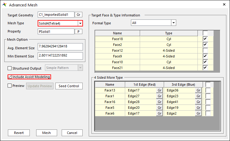
In the Advanced Mesh dialog window, perform the following:
In the Mesh Type dropdown menu, select Solid4 (Tetra4).
Select the Include Assist Modeling checkbox.
Tip
You must select this to ensure that the FDRs are automatically generated according to the conditions defined in Assist Modeling.
Click Mesh.
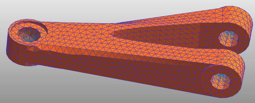
Once Meshing is complete, click Close.
The mesh model of the UCA body appears, as shown below.
Tip
RecurDyn offers two auto-meshers, Mesh and Advanced Mesh. The Mesh auto-mesher applies tessellation to the geometry in the GUI before generating the mesh. The Advanced Mesh auto-mesher skips the tessellation stage altogether and generates the mesh directly. By doing so, Advanced Mesh minimizes the distortion of the CAD geometry. However, Advanced Mesh also increases the Mesh failure rate.
Perform either of the following steps to return to the parent mode:
Right-click the Working window, and from the menu that appears, click Exit.
From the Exit group in the Mesher tab, click the Exit function.
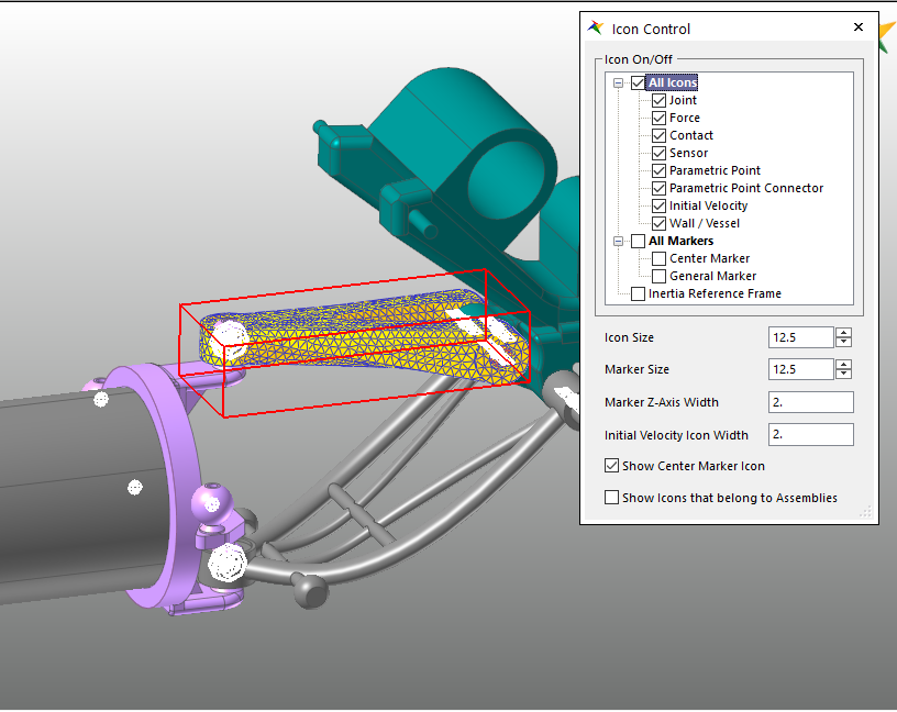
Note that the existing UCA Rigid Body (UCA) disappears and it is replaced by the UCA Flexible body (UCA_FE). Also, the joint and the force previously created are maintained as they were in the GUI. At this moment, to see the icons, click the Icon Control tool on Render Toolbar and select All Icons.
To check if the modeling is correctly configured for the UCA Flexible body, return to the Assembly mode and run Dynamic Analysis using the previous conditions. The analysis will be completed quickly.
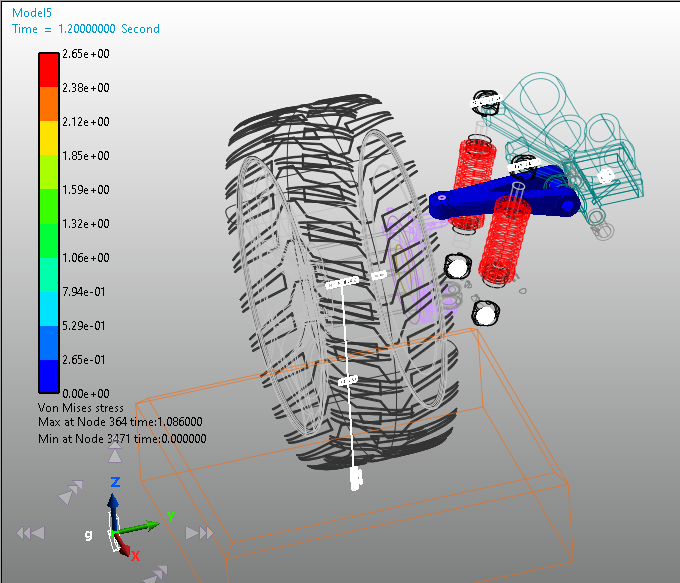
From the FFlex group in the Flexible tab, click the Contour function to view the results.
8.3.3.4. Creating an LCA Body Mesh
In Assembly mode, double-click the Suspension_Assy created as a subsystem to enter the Subsystem mode.
In Subsystem mode, select the body and the LCA body. Right-click the selected body, and select Mesh from the context menu, as shown in the figure to the below.
The LCA body appears as shown in the figure below.
In Mesh mode, click the Assist Modeling function from the Mesher group in the Mesher tab. The Assist Modeling dialog window appears.
In the Add/Remove column of the dialog window, click Gr to assign the geometries for the areas where the Slave Nodes will be created. Referring to the following page, select the geometries where the slave nodes will be created for three FDRs.
Tip
When you click Gr, a marker appears on the screen indicating where the master node will be generated. This helps you locate the areas to assign slave nodes.
Tip
Due to the nature of the FDR, the master node is automatically generated at the point where the joint and the force are created. You must define the slave nodes directly.
After all the geometries are assigned, right-click the model, and click Finish Operation.
For the other four areas, select the Surfaces where the Slave Nodes will be created, as shown in the figures below:
Once you have selected all the geometry items, click OK.
From the Mesher group in the Mesher tab, click the Geometry Refinement function.
Tip
The geometry refinement function is only effective when using the mesh method. That is, as with the UCA body, if the advanced mesh method is used, then it has no effect at all.)
The Geometry Refinement dialog window appears.
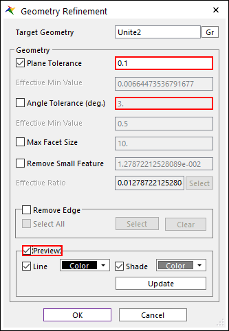
In the Geometry Refinement dialog window, change the Plane Tolerance to 0.1.
In the Geometry Refinement dialog window, check out the Angle Tolerance.
Select the Preview checkbox. The tessellated shape appears, as shown in the figure to the below.
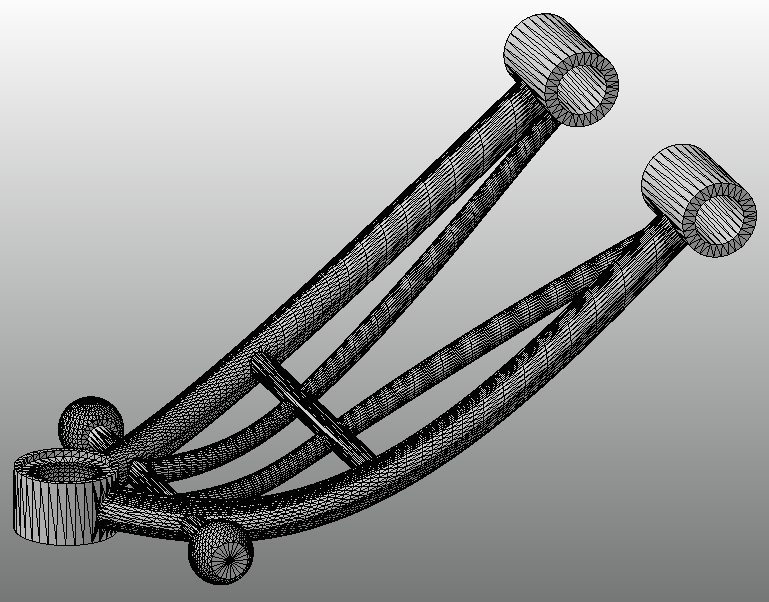
Click OK to close the dialog window.
Tip
RecurDyn features two Auto-Meshers, Mesh and Advanced Mesh. The Mesh auto-mesher applies tessellation on the geometry in the GUI before generating the mesh. The Advanced Mesh auto-mesher skips the tessellation stage altogether and generates the mesh directly. The LCA body has a lot of curved surfaces, so you should use the Mesh auto-mesher (which applies tessellation) to reduce the number of nodes. The geometry refinement function used for the LCA body applies the tessellation and has nothing to do with the Advanced Mesh method.
Click the Auto Mesh function. The Mesh dialog window appears.
In the Mesh dialog window, perform the following:
Select Solid4 (Tetra4) as the Mesh Type, as shown in the figure to the below.
In the Mesh Option group, set the Max Element Size to 4 and the Min Element Size to 2.
Select the Include Assist Modeling checkbox.
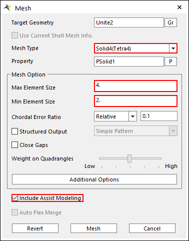
Click Mesh.
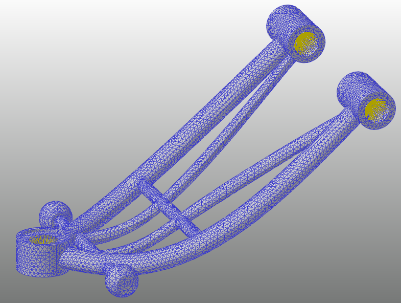
The mesh model and FDR of the LCA body are created, as shown in the figure below.
Perform either of the following steps to return to the parent mode:
Right-click the Working Window, and from the menu that appears, click Exit.
From the Mesher group in the Mesher tab, click the Exit function.
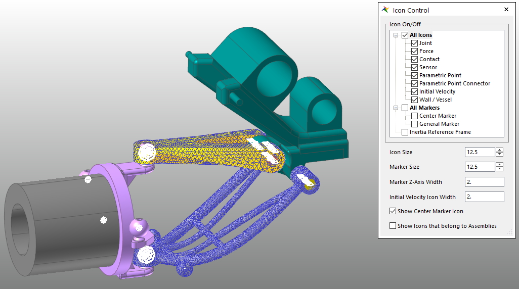
Note that the existing LCA Rigid Body (LCA) disappears and it is replaced by the LCA Flexible body (LCA_FE), as shown in the figure below. Also note that the joint and the force previously created are maintained from the GUI. At this point, to see the icons, click the Icon Control tool in Render Toolbar and select the All Icons checkbox.
To check if the modeling is correctly configured for the created LCA Flexible body, Exit to the Assembly mode and run the Dynamic Analysis under the previous conditions. The analysis will take a little longer than in the previous step, but it will not take too long to produce the results. From the FFlex group in the Flexible tab, click the Contour function to produce the results shown below.
8.3.4. Conducting Durability Analysis
8.3.4.1. Task Objective
This chapter teaches you how to analyze the durability of an FFlex body.
8.3.4.2. Estimated Time to Complete
40 minutes
8.3.4.3. Conducting a Durability Analysis on the UCA_FE Body
8.3.4.3.1. To create a patch set:
In Assembly mode, double-click the Suspension_Assy to enter Subsystem mode.
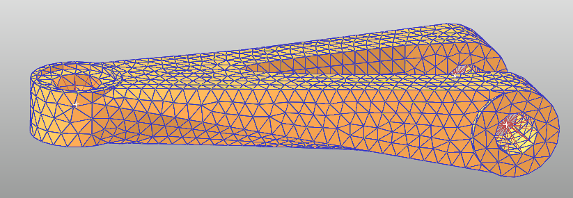
Double-click the UCA_FE body to proceed to the Body Edit mode.
From the Set group in the FFlex Edit tab, click the Patch Set function.
Click the Add/Remove button, as shown below. Click and drag the mouse button to select the entire body.
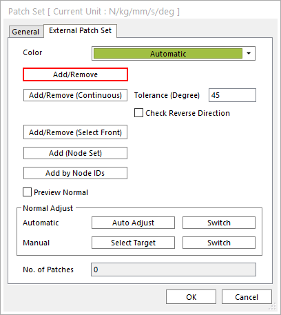
Right click the body and click Finish Operation in the context menu.
In the Patch Set dialog window, click OK.
Confirm that the patch set is created and click the Exit function from the Exit group in the FFlex Edit tab to return to the parent mode.
To set the patch set for the LCA_FE body, repeat steps 2 to 7.
When you have completed the above procedures, the patch sets have been created for each of the two Flexible Bodies.
Right-click the Working window, and from the menu that appears, click Exit to return to the Assembly mode.
8.3.4.3.2. To retrieve the animation file:
From the Animation Control group in the Analysis tab, click the Reload the last animation file function.
Note that all of animation-related buttons are activated.
Tip
8.3.4.3.3. To set the analysis preferences:
From the Durability group in the Post Analysis tab, click the Preference function.
- In the Preferences dialog window, on the Material page, specify the path of the Material Library file for the Fatigue Analysis.(C:\Users\<Your Windows Login ID>\Documents\RecurDyn\<RecurDyn Version>\Durability or the equivalent path).
On the Fatigue Influencing Factors page, in the Fatigue Factors group, set the Notch Factor Amp (Kf, Kt) to 2, as shown below.
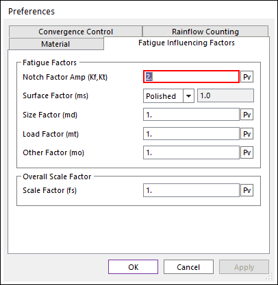
The Notch Factor increases the analytically derived stress value to account for stress concentrations due to the cracks, holes, and notches (V grooves) caused by the design and processing of the structure. Therefore, the larger the notch factor value is, the more severe the durability analysis will be.
Tip
For reference, the values included in the Fatigue Influencing Factors represent the physical conditions of actual test samples in an actual durability analysis experiment, so they all have default values of 1. Modifying each factor varies the S-N curve accordingly: making it possible to simulate more severe conditions in the durability analysis.If the values other than the notch factor are less than 1 and the notch factor value is greater than 1, then the conditions simulated in the durability analysis will be more severe.In the Preferences dialog window, do not change the Convergence Control and Rainflow Counting values, and click OK.
8.3.4.3.4. To conduct the fatigue evaluation:
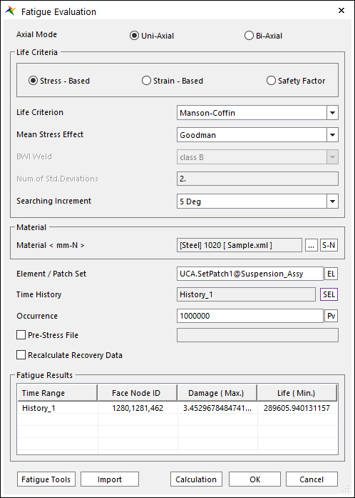
From the Durability group in the Post Analysis tab, click the Fatigue Evaluation function. The Fatigue Evaluation dialog window appears.
In the Fatigue Evaluation dialog window, perform the following:
Set the Axial Mode to Uni-Axial.
Set the Searching Increment to 5 Deg.
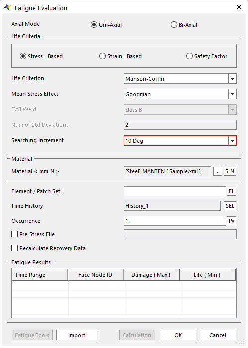
In the Material group, click …. The Material Manager dialog window appears.
In the Material Manager dialog window, perform the following:
Select and right-click [Steel] 1020, and click Make Active in the context menu, as shown in the figure to the below.
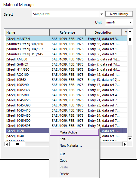
Click OK.
In the Element/Patch Set group, click EL.
Select the set Patch Set for the UCA_FE body.
Since the UCA_FE body is included in the Suspension_Assy subsystem, you must click the UCA_FE body button while pressing the Shift key. As a result, UCA_FE.SetPatch1@Suspension_Assy will appear on the Element/Patch Set item.
Click the SEL button in the Time History text box.
A Time History set is defined already, in the Time History dialog window. To change the range of time, click R.
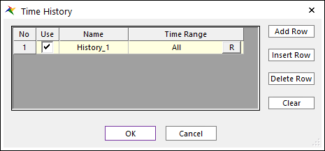
In the Time Range dialog window, click All.
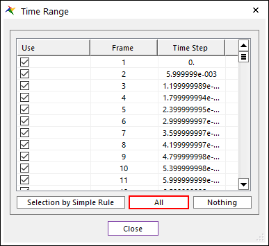
Click Close in the Time Range dialog window.
Click OK
In the Occurrence text box, type 1000000.
Click Calculation.
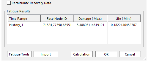
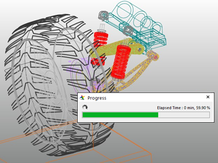
A Progress Bar appears to display the fatigue analysis progress. Upon completion of the analysis, the results will appear in the results group, as shown in the figure to the below.
In the Fatigue Evaluation dialog window, click Fatigue Tools.
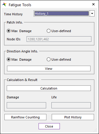
Click Rainflow Counting in the Fatigue Tools dialog.
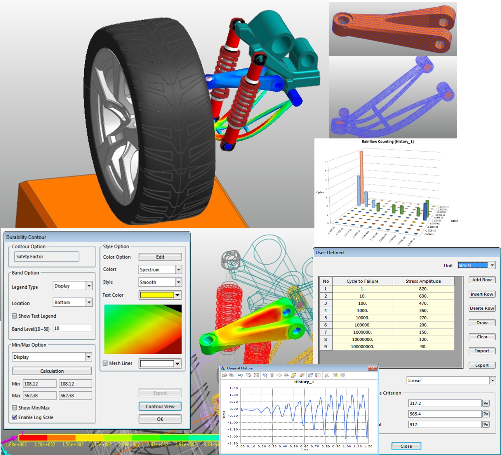
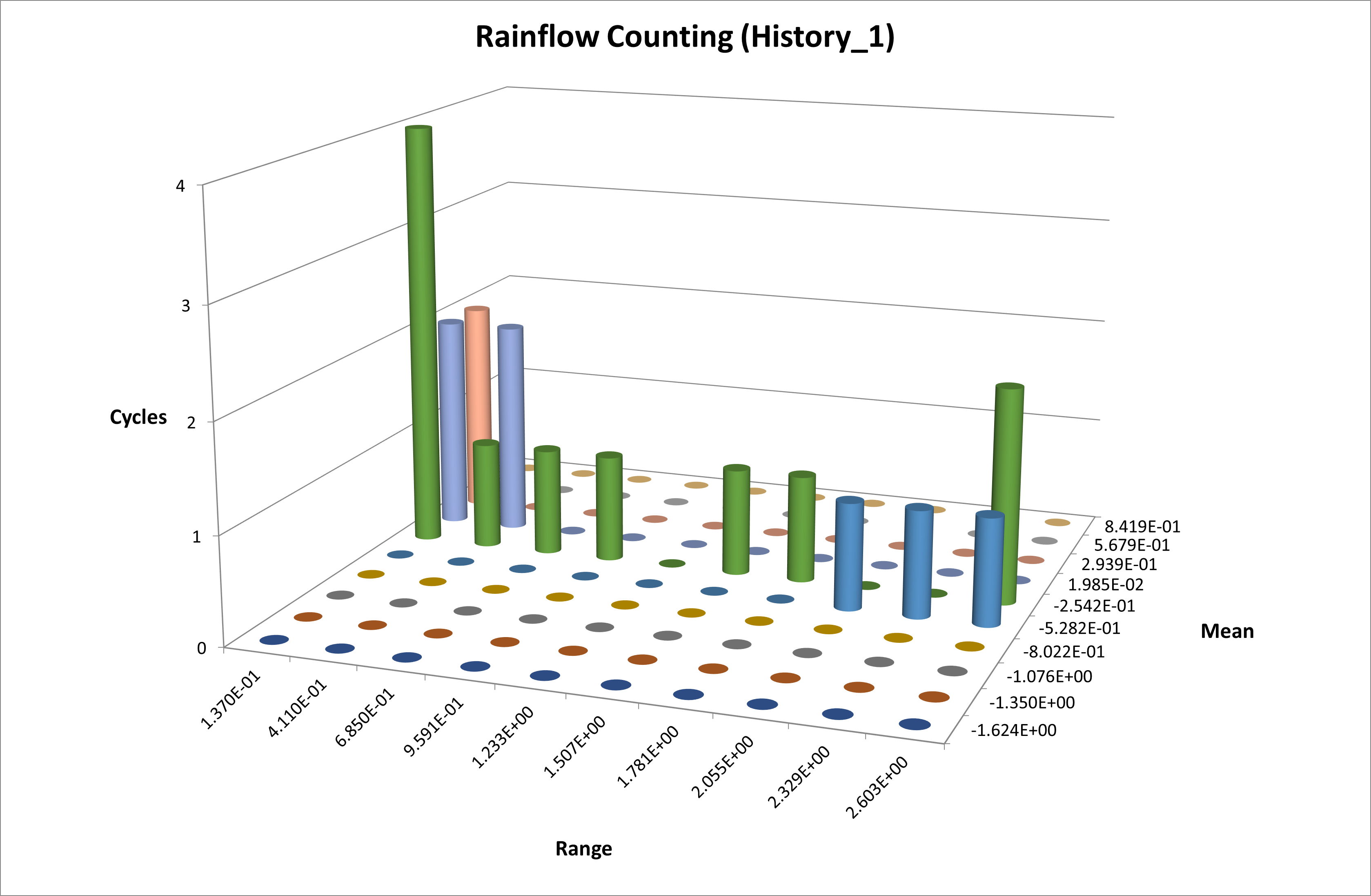
As shown below, the Rainflow Counting results in the Excel are based on the Stress Time History applied to the patch zone where the damage is largest. The results are displayed in the numbers of cycles according to the stress amplitude and the mean stress.
Click the Plot History in this dialog.
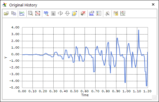
As shown below, it is possible to check the Stress Time History on the patch which has the maximum damage results among the defined patches.
8.3.4.3.5. To verify the contour results:
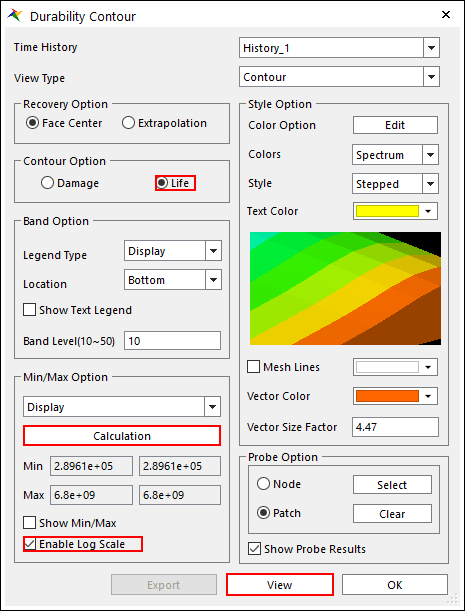
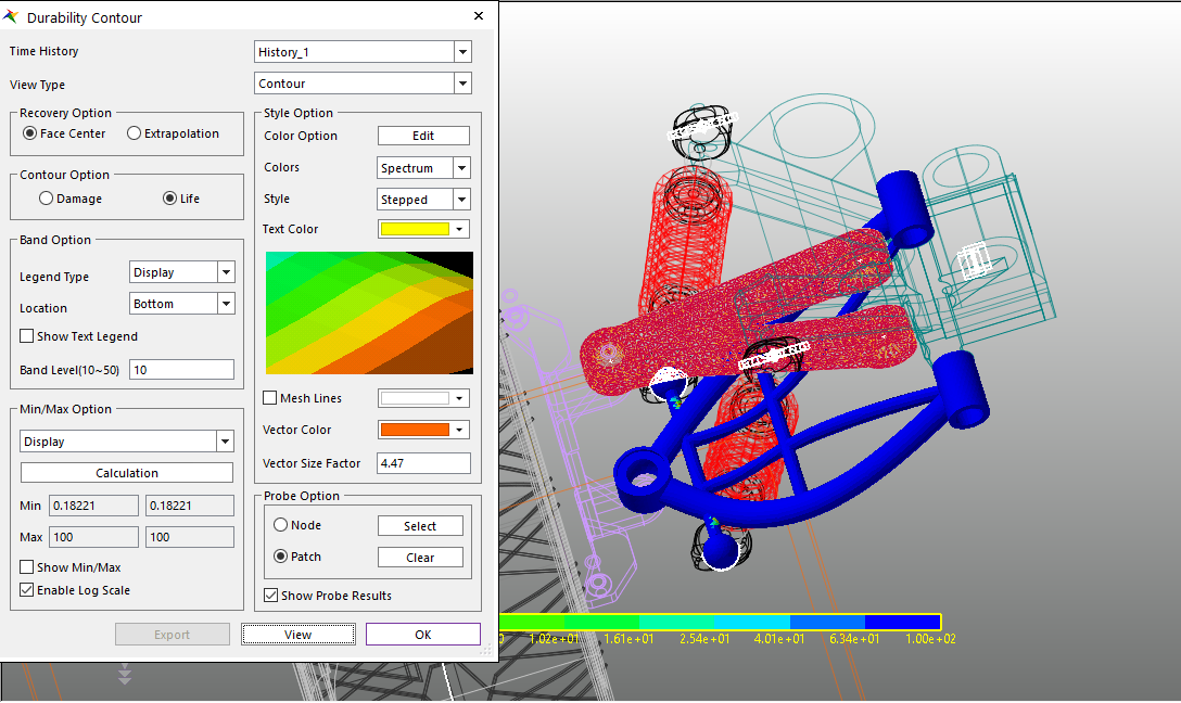
From the Durability group in the Post Analysis tab, click the Contour function. The Durability Contour dialog window appears.
In the Durability Contour dialog window, perform the following:
In the Contour Option group, select Life.
Click Calculation.
Select Enable Log Scale.
Click Contour View to view the results.
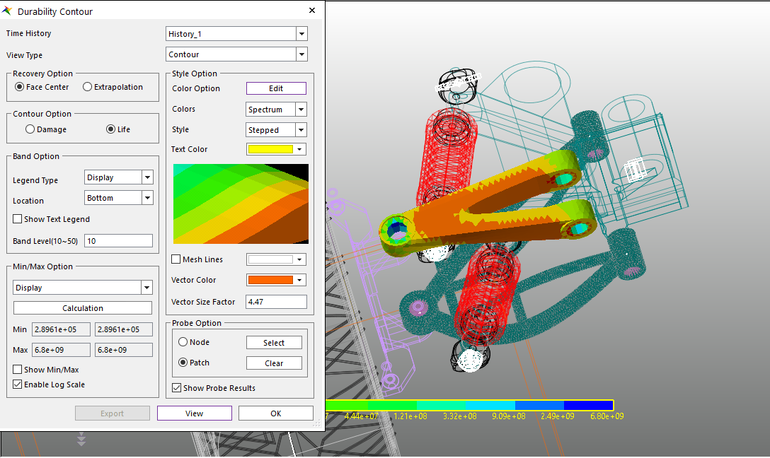
To make the results more visible, click Edit in the Style Options group of the Durability Contour dialog window, and change the colors as follows.
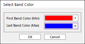
Click Contour View again to highlight the least durable sections in red, as shown below. This makes it easier to identify the areas with a relatively short fatigue life.
Tip
At this point, if you would like a more detailed Contour Plot, then select Wireframe in the toolbar before viewing the results.
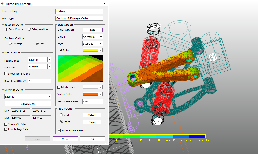
Select Contour & Damage in the View Type on options in order to check the damage direction on each patch.
As shown below, if the View button is pushed, the damage direction will appear.
8.3.4.4. Conducting a Durability Analysis on an LCA_FE Body
8.3.4.4.1. To set the analysis preference:
From the Durability group in the Post Analysis tab, click the Preference function. The Preference dialog window appears.
In the Preference dialog window, perform the following:
On the Fatigue Influencing Factors page, in the Fatigue Factors group, change the Notch Factor Amp (Kf, Kt) from 2 to 1.

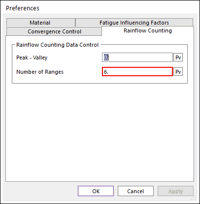
On the Rainflow Counting page, in the Rainflow Counting Data Control, change the Number of Ranges to 6.
Tip
At this point, if you change the number of ranges when running Rainflow Counting in the Fatigue Evaluation dialog window and set the number of cycles on mean stress and stress amplitude, then the number of ranges for the mean stress and stress amplitude in the Excel chart will be the value you have set.
8.3.4.4.2. To use a user-defined S-N curve:
From the Durability group in the Post Analysis tab, click the Fatigue Evaluation function. The Fatigue Evaluation dialog window appears.
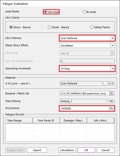
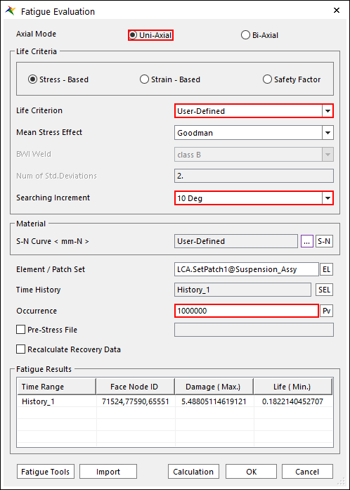
In the Fatigue Evaluation dialog window, perform the following.
Change the Axial Mode to Uni-Axial.
In the Life Criteria group, select User-Defined.
Set the Searching Increment item to 10 Deg.
Set the Occurrence to 1000000.
In the Material group, click …. The User-Defined dialog window appears.
In the User-Defined dialog window, perform the following:
Click the Add Row button 9 times, and enter the values shown in the figure to the below.
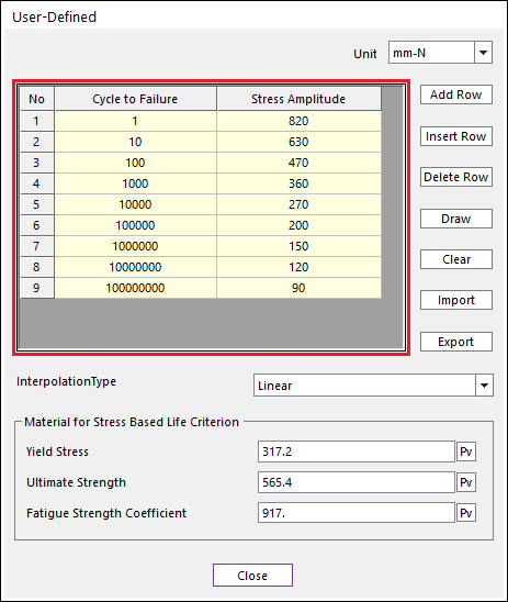
Click Draw to show the S-N curve for the given values.
Click Close.
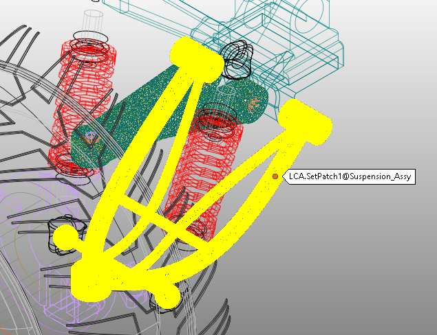
In the Element/Patch Set group, click EL.
Select Patch Set for the LCA_FE body.
Return to the Fatigue Evaluation dialog window and note that the Element/Patch Set item maintains the patch data of the UCA_FE body set in the previous step. For this tutorial, however, hold down the Shift key and select the patch data that was defined as the LCA_FE body, as shown in the figure below.
Click Calculation.
The Fatigue Analysis processing status appears in a Progress Bar, as shown below.
When the Fatigue Analysis is complete, the Fatigue Evaluation dialog window displays the Maximum Damage and Minimum Life.
In the Fatigue Evaluation dialog window, click Fatigue Tool.
As shown below, the Rainflow Counting results displayed in the Excel file are based on the Stress Time History applied to the patch zone where the damage is the largest. Unlike the Rainflow Counting result for the UCA_FE body, there are 6 ranges in the 3D chart because you changed the number of ranges in the Rainflow Counting data set to 6 in the Preference dialog window.

Open the Contour dialog window, and select Life in the Contour Option group, as you did when verifying the durability analysis results for the UCA_FE body.
Click Calculation and note that the Min/Max values are calculated in the dialog window. Then, click Contour View to display the results, as shown below.
8.3.5. Analyzing and Reviewing Results
8.3.5.1. Task Objective
This chapter teaches you how to analyze and review the durability results of the two models.
8.3.5.2. Estimated Time to Complete
5 minutes
8.3.5.3. Analyzing Durability Results
8.3.5.3.1. Analyzing the results for the UCA_FE body
Before conducting the durability analysis, if you compared the Von-Mises stresses for the UCA_FE and LCA_FE bodies after the final step in Chapter 3, then the stress generated in the UCA_FE body would be relatively low. Therefore, you would anticipate that its durability would be very high as well. However,
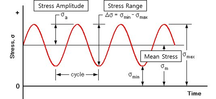
In actuality, the rainflow counting result derived from the stress time history used in the fatigue analysis, shown in the figure below, reveals that the largest stress range (where the stress range is twice the stress amplitude) repeatedly added on the weakest point (the patch zone) is about 2.6 Mpa and the mean stress is less than 0.841 Mpa.

For reference, the relationship between the stress amplitude, stress range, mean stress, and cycle are shown in the stress time history below.
As you can see from the simulation results, the load was applied to the UCA_FE body repeatedly in the same direction and our durability analysis used the Uni-Axial for the axial type. Since the loads were added a million times during the simulation (occurrence = 1,000,000), this stress life criteria assumes a highly repetitive life. Therefore, the mean stress effect was applied here.
The durability analysis also used 1020 series steel (available in the Durability Material Library), which is largely used in the vehicle structures.
The results indicate that the repetition number for the most damaged section, which is the section with the shortest fatigue life. In other words, under the load conditions of the simulation, Fatigue Evaluation is the value obtained by multiplying Occurrence condition and fatigue life.
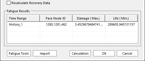
Assuming that the fatigue life result shown above has an infinite life, then you can apply the safety factor to the life criteria to derive another fatigue analysis result for the UCA_FE Body design.
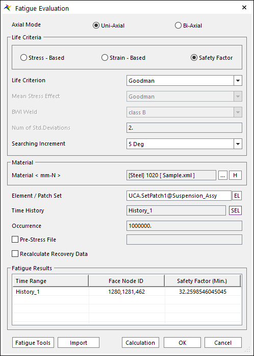
To do so, select Safety Factor for Life Criteria only, and leave the searching increment, element/patch set, and materials the same as those applied to the UCA_FE body. This will produce the results shown below. (Tip: At this point, change the notch factor to 2 in the Preference dialog window.)
Select this option in the Contour Plot to produce the following results.
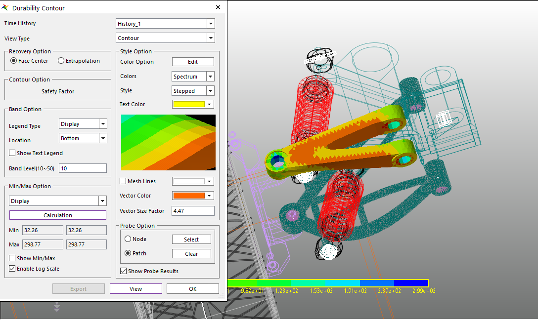
The conditions required in the Safety Factor calculation are the stress amplitude and the mean stress from the Rainflow Counting results. Therefore, the occurrence data related to the number of cycles is unnecessary. The durability analysis results shown above reveal that the UCA_FE body is very stable.
8.3.5.3.2. Analyzing the results for the LCA_FE body
Unlike the UCA_FE body, you must enter the formulas for the durability analysis of the LCA_FE body instead of using the ones provided by RecurDyn/Durability, which create specific S-N Curves. This means that you can directly input data obtained from external experiments and/or related resources (stress amplitude vs. cycle) when setting the materials for the fatigue analysis by selecting User-Defined S-N Curve.
As you can see in the rainflow counting results graph, the stress range and the mean stress are approximately 40 times larger than the results obtained for the UCA_FE body.

You can conclude from the fatigue analysis results that the LCA body can survive only up to 1 million times under the given load conditions. Therefore, a design change is essential in order to make the product more durability.
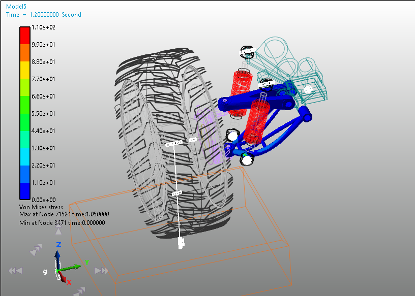
If you were to determine the stability of the LCA_FE Body based on the Von-Misess stress only, then the maximum stress would be about 137 Mpa, as shown below, which is less than the yielded stress (262 Mpa). Therefore, this design could be considered stable. As far as durability is concerned, however, it is necessary to alter the design.