3.7. Connecting Rod Shape Optimization Tutorial (AutoDesign)

3.7.1. Connecting Rod Shape Optimization

This tutorial deals with the shape optimization design problem. Design target is a connecting rod in engine. Connecting rod function is a transferred reciprocating movement of the piston to crankshaft rotational movement. Therefore, design goal is a minimize mass for energy efficiency and reduce inertial force. Also, a design constraint is strength to withstand compressive forces of piston. Design variables select the shape on connecting rod.

Open files related in Sample-G
Sample	<InstallDir>\Help\Tutorial\AutoDesign\ConnectingRodShape\Examples\Sample_G.rdyn
Solution	<InstallDir>\Help\Tutorial\AutoDesign\ConnectingRodShape\Solutions\Sample_G.rdyn

Note

If you change the file path at discretion, it can be located in any folder that you specify.

3.7.2. Loading and simulation the model

1. On your Desktop, double-click the RecurDyn icon. RecurDyn starts and the Start RecurDyn dialog box appears.

2. Close Start RecurDyn dialog box. You will use an existing model.

3. In the Quick Access Toolbar, click the Open tool and select Sample_G.rdyn from the same directory where this tutorial is located.

   The system appears on the screen.
   

4. Click Dynamic/Kinematic.

5. Click Simulate.

6. In order to view result, click play.

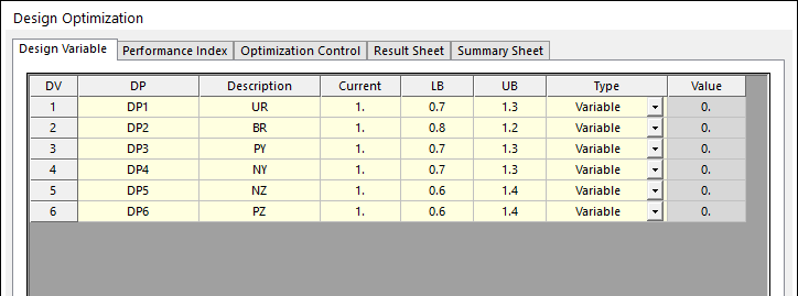
3.7.3. Defining the design variables and setting

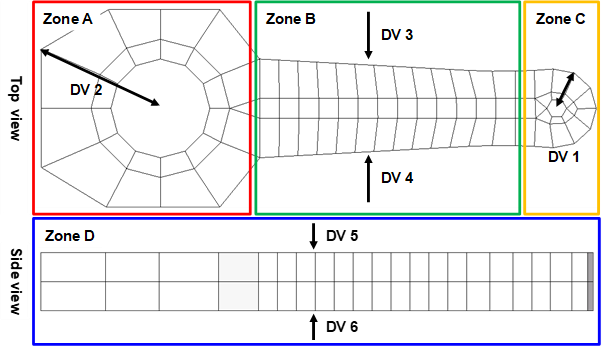
In the figure, design variable selects connecting road shape. Design variables divide into 4 design variable zones. And DV1 is a radius in zone C and DV2 is radius in zone A. DV3 and 4 is a width in zone B. DV 5 and 6 is a height in zone D.

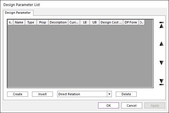
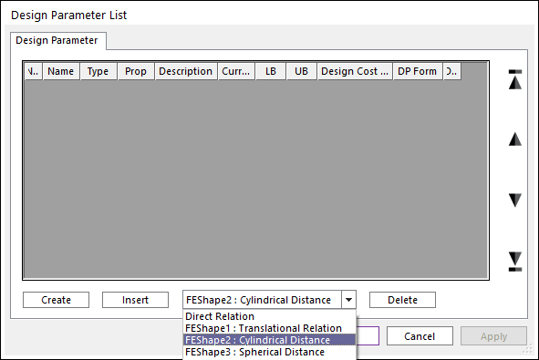
1. From the Auto Design menu, click Design Parameter. This will bring up the design parameter list dialog as shown below.

   

2. To set design variable 1

   1. Select design parameter type as FEShape2: Cylindrical distance. And click Create to add design parameter. This will bring up the FEShape 2: Cylindrical distance window shown below.

      

   2. Node set: UR in zone C

      

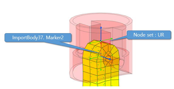
   3. Configuration design: off

   4. Center Reference marker: importbody37.Marker2

   5. Center Axis: 0,0,1

   6. Lower & upper bound: 0.7,1.3

   7. OK

      

3. To set design variable 2

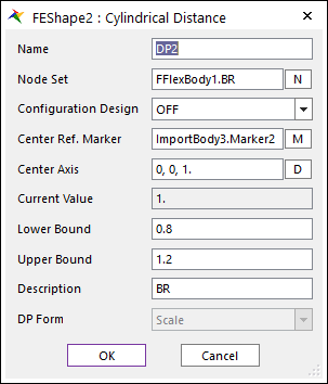
   1. Select design parameter type as FEShape 2: Cylindrical distance. And click Create to add design parameter.

   2. Node set: BR in zone A

      

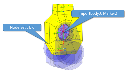
   3. Configuration design: off

   4. Center Reference marker: importbody3.Marker2

   5. Center Axis: 0,0,1

   6. Lower & upper bound: 0.8,1.2

   7. OK

      

4. To set Design variable 3, 4

   1. Select design parameter type as FEShape 1: Translational relation. And click Create to add design parameter. This will bring up the FEShape 1: Translational relation window shown below.

   2. Node set: PY in Zone B

      

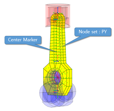
   3. Configuration design: off

   4. Reference marker: Flexbody1.CM

   5. Directional unit vector: 0,1,0

   6. Lower & upper bound: 0.7,1.3

   7. OK

   8. In like manner, To generate DV4 about node set:NY

      

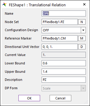
5. To set Design variable 5, 6

   1. Select design parameter type as FEShape 1: Translational relation. And, click Create to add design parameter.

   2. Node set: NZ in zone D

      

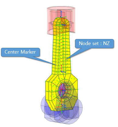
   3. Configuration design: off

   4. Reference marker: Flexbody.CM

   5. Directional unit vector: 0,0,1

   6. Lower & upper bound: 0.6,1.4

   7. OK

   8. In like manner, To generate DV6 about node set: PZ

      

3.7.4. Defining the analysis responses

In order to design connecting rod, analysis response is a mass and stress

1. Click the Analysis Responses menu. Then, you can change the response type (FE-Result) as follow figure:

   

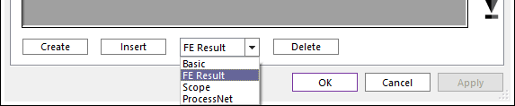
2. Click the Create button. Then you can see the Analysis Responses-FE Result window as following figure.

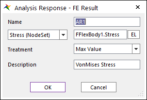
3. To set the analysis response of stress is defined as

   1. Name: AR1

   2. Result type: Stress(NodeSet)

   3. Select Node Set: FFlexBody1.Stress

   4. Response treatment: Max value

   5. Description: VonMises Stress

   6. OK.

      

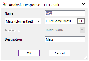
4. Click the Create button. Then you can see the Analysis Responses-FE Result window as following figure.

5. To set the analysis response of mass is defined as

   1. Name: AR2

   2. Result type: Mass(ElementSet)

   3. Select Element Set: FFlexBody1.Mass

   4. Description: Mass

   5. OK.

      

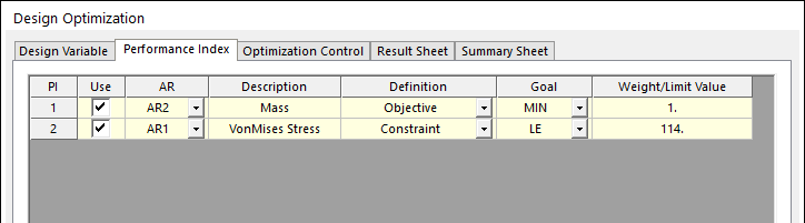
3.7.5. Running a design optimization

The optimization problem is defined as:

Minimize the mass of the connecting rod

Subject to

• The stress =< Limit value

1. Click the Design Optimization menu. Then, you can see the design variable list as following figure:

   

2. Click the Performance Index tab. Then, you can see the following list. If this window is empty, then you create the following PIs.

   

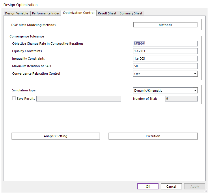
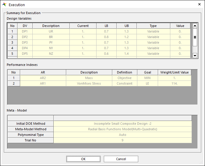
3. Click the Optimization Control tab. The default values are directly used. Then, click Execution. Then, you can see the summary of design formulation. Check design variables, performance index and Meta-Model information. If all information is correct, then click OK. Then, optimization process is progressed.

   

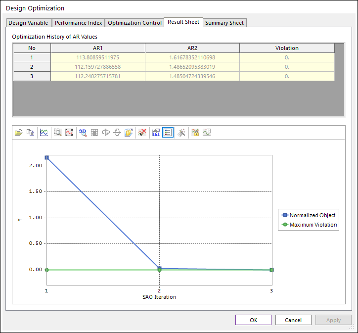
4. When the optimization process is completed, the Result Sheet page is automatically shown. The optimization process is converged only in 5 iterations. Thus, AutoDesign solves the connecting-rod system design having 6 design variables for 12 analyses that includes 9 analyses for the initial sampling points. The final design gives that AR1=112.2 Mpa and AR2=1.485 kg which can minimize the Mass by 58 % and the stress is satisfied with design constraint (less than 114 Mpa).

   

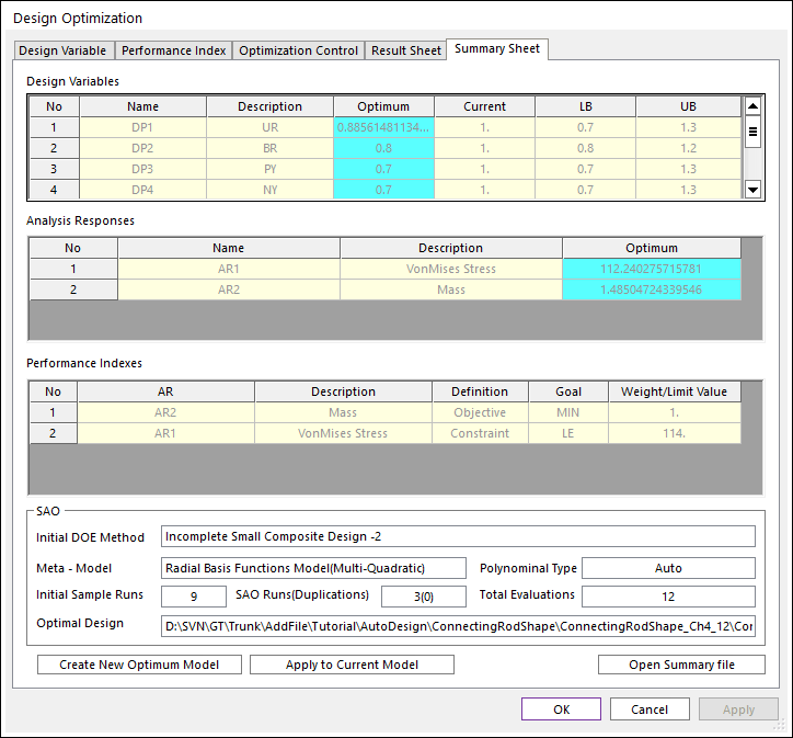
5. The optimization results are summarized in the design variables and analysis responses lists. Also, the SAO information is summarized, which shows that SAO 5 requires. The analysis result of optimal design is DO_005.

   

3.7.6. Comparison of analysis results

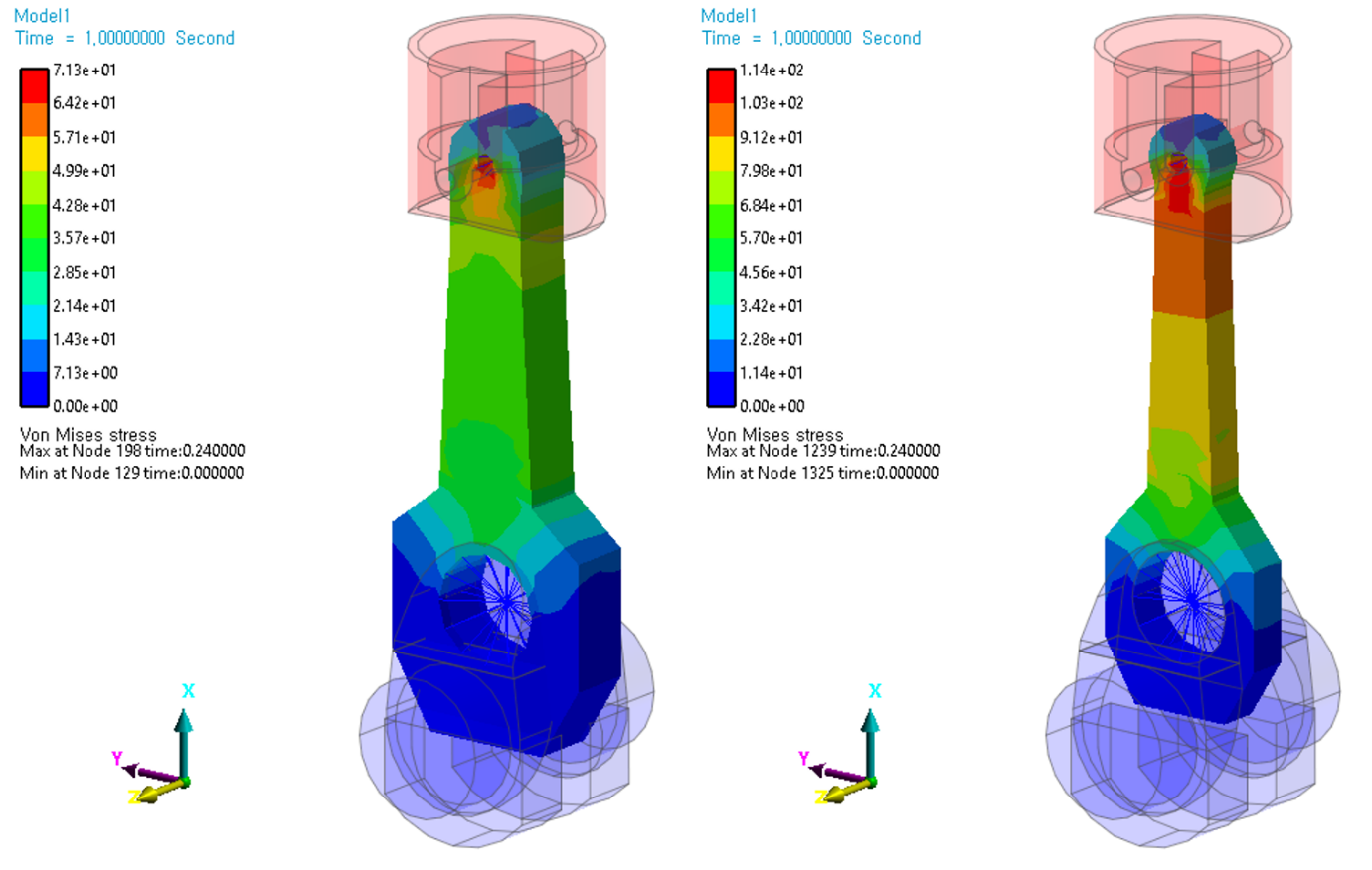
Finally, let’s compare the mass and stress level for the initial design and the optimal design. SAO3 is the optimal design. Also, DOE009 is the initial design. The following figures show those comparisons.

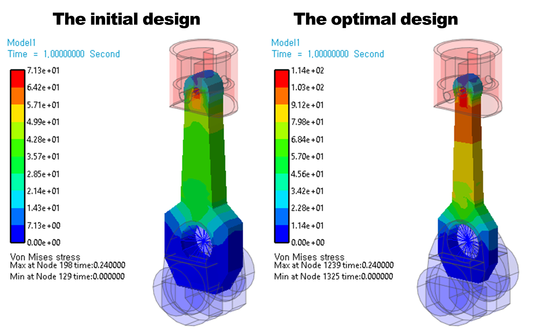
	The initial design	The optimal design
Mass (Kg)	3.478	1.485
Stress (Mpa)	71.3	112.2