9.4. Gearbox Tutorial (DriveTrain)

9.4.1. Getting Started

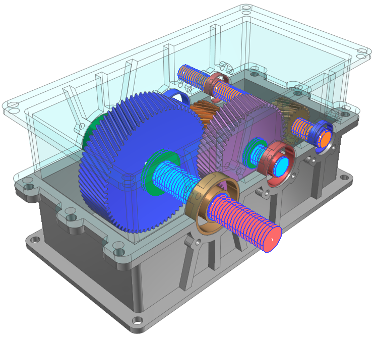
DriveTrain Toolkit can design the mechanical system composed of shaft, gear, bearing, etc. It can consider the material and dynamic properties of its parts. For shaft, it can design and analyze the shaft with the various radii using the FE Beam Element. For gear, it co-simulates with KISSsoft for more accurate and detailed result and it can be used with Involute Analytic Gear Contact for reduced simulation time with accurate result. For bearing, it also co-simulates with KISSsoft for more accurate and detailed result.

In this tutorial, you will learn about the process of simulation of gearbox system using DriveTrain Toolkit. You can learn how to use the new functions and analyze the simulation results.

9.4.1.1. Objective

You will also learn below.

Create a shaft, bearing, gear
Create an analytic gear contact
Analyze the simulation result of shaft, bearing, gear

9.4.1.2. Prerequisites

This tutorial is for the users who already learned the basic tutorial and the FFlex tutorial. Therefore, you should first work through the tutorials that mentioned earlier to enhance the understanding of this tutorial. Also, we assume that you have a basic knowledge of dynamics and the Finite Element Method.

9.4.1.3. Procedures

This tutorial is comprised of the following procedures. The estimated time to complete each procedure is shown in the table below.

Procedures	Time (minutes)
Simulation environment setup	10
Create shaft	10
Create bearing	10
Create gear	15
Create joint, force	20
Analyze the simulation result	20
Create involute analytic contact	20
Total	105

9.4.1.4. Estimated Time to Complete

1 hours and 45 minutes

9.4.2. Setting Up the Simulation Environment

9.4.2.1. Task Objective

In this chapter, you will start the RecurDyn and setup its environment, including importing the completed gearbox CAD and changing its names and layer.

9.4.2.2. Estimated Time to Complete

15 minutes

9.4.2.3. Starting the RecurDyn

9.4.2.3.1. To start the RecurDyn and create a new model:

On your Desktop, double-click the RecurDyn icon and the New Model dialog box will appear.
Change the Model Name to GearBox.
Ensure the units are the same as those in the Start RecurDyn dialog box. If not, click MMKS. (Millimeter/Kilogram/Newton/Second)
Click OK.

9.4.2.4. Importing the Gearbox Geometry

You will begin to model the gearbox by importing an already completed gearbox CAD.

9.4.2.4.1. To import the gearbox CAD

From the File menu, Choose the Import function.
In the Open dialog box, select the file GearBoxCAD.x_t.

(The file path: <InstallDir>\Help\Tutorial\Toolkit\DriveTrain\GearBox)
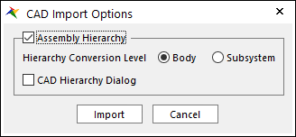
Click Open. The CAD Import Options dialog appears. Make sure the option Assembly Hierarchy is checked and the option Body is checked in the Hierarchy Conversion Level and click Import.

9.4.2.4.2. To change the name of CAD and set layer

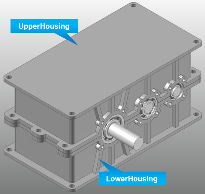
Right-click the Upper Housing body as shown in the figure below and click Properties in the Pop-up menu.
In the General page, you will adjust the value using the information below and click OK.
- Name: UpperHousing
- Layer: 2
For the Lower Housing body, change the Name to LowerHousing and Layer to 2.

9.4.2.5. Adjusting the Icon, Marker Size and Layer

9.4.2.5.1. To adjust the icon and marker size

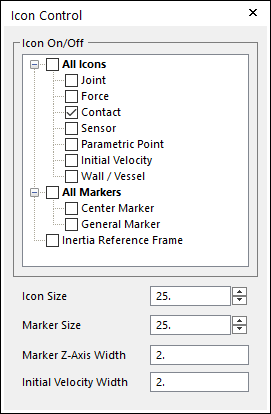
In Render Toolbar, click the Icon Control tool as shown in the figure below.
Set the Icon Size and Marker Size to 25 as shown at below.

9.4.2.5.2. To adjust the layer setting

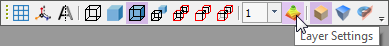
In Render Toolbar, click the Layer Settings tool as shown in the figure below.
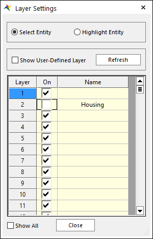
Change the Name of Layer 2 to Housing and Check Off the Layer On option as shown at below.

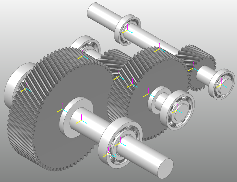
The model appears as shown in the figure below.

9.4.2.6. Saving the Model

Take a moment to save your model before you continue with the next chapter. (From File menu, click the Save function.)

9.4.3. Creating the Shaft

9.4.3.1. Task Objective

In this chapter, you will learn how to use the shaft modeler that can create various types of shaft sections which are composed of finite beam element with different circular cross sections.

9.4.3.2. Estimated Time to Complete

10 minutes

9.4.3.3. Creating the Shaft

You will create the shaft with beam element to analyze the stress and deformation of shaft in gearbox system.

9.4.3.3.1. To create the Shaft1

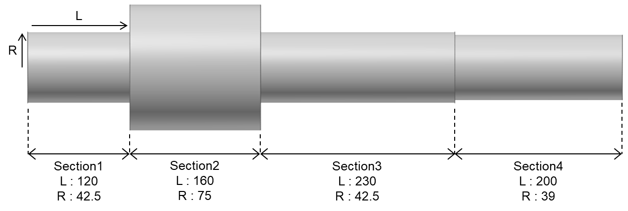
Shaft Modeler in RecurDyn defines the section as parts with same radius, length and material. Number of shaft section increases from starting point towards axial direction. Design of the Shaft1 is shown in the figure below.

From the Shaft group in the DriveTrain tab, click the Shaft function.
Set the Creation Method to Point, Direction, WithDialog and input the value using following information.
- Point: -255, 250, 175
- Direction: 1, 0, 0
After Shaft dialog appears, click Add 3 times to make 4 Sections and adjust the values using following information.

Section

L

Ro

Ri

Element Size

1

120

42.5

0

10

2

160

75

0

10

3

230

42.5

0

10

4

200

39

0

10
Click FDR which is located next to the Sections box. After FDR dialog appears, click Add button 3 times to make 3 FDRs and adjust the values using the following information.

No

Center Position

Width

Type

1

22.5

41

RBE2

2

200

120

RBE2

3

487.5

41

RBE2
Click Close to exit FDR dialog.
Click OK to create Shaft.
Delete the existing Shaft body where Shaft1 has been created.

Note

FDR

Most of the time Shafts are attached with the machine elements like gear, bearing, etc. Connectors like pin, key, spline, snap ring are used to attach those elements. In RecurDyn, connections of these machine element are expressed as FDR element which is rigid element.

If you look at the center position of the FDR which is master node, you can see that the size of master node is bigger than the size of other nodes.

FDR Tolerance

When you create a FDR element, 3 nodes, center position and two end sides of FDR, are added to the existing nodes. The distance between existing node and the added FDR node can be very small. The FDR Tolerance is used to ignore the small element caused by creation of FDR.

For example, if FDR Tolerance is 0.01 and the distance between two nodes are 0.009, the added FDR Element is ignored and altered as existing node.

9.4.3.3.2. To create the Shaft2

Create the Shaft2 using same method as above using the following information.

Point, Direction, WithDialog
- Point: -255, 250, -105
- Direction: 1, 0, 0
Shaft Section

Section

L

Ro

Ri

Element Size

1

50

32.5

0

10

2

235

37.5

0

10

3

125

50

0

10

4

100

32.5

0

10
FDR Section

No

Center Position

Width

Type

1

22.5

33

RBE2

2

200

120

RBE2

3

347

90

RBE2

4

487.5

33

RBE2

9.4.3.3.3. To create the Shaft3

Create the Shaft3 using same method as above using the following information.

Point, Direction, WithDialog
- Point: -402, 250, -325
- Direction: 1, 0, 0
Shaft Section

Section

L

Ro

Ri

Element Size

1

657

30

0

10
FDR Section

No

Center Position

Width

Type

1

169.5

22

RBE2

2

494

90

RBE2

3

634.5

22

RBE2

The model appears as shown in the figure below.

9.4.3.4. Saving the Model

Take a moment to save your model before you continue with the next chapter. (From File menu, click the Save function.)

9.4.4. Creating the Bearing

9.4.4.1. Task Objective

In this chapter, you will learn how to create a Ball Bearing using a KISSsoft Ball Bearing Library.

9.4.4.2. Estimated Time to Complete

10 minutes

9.4.4.3. Creating the Bearing

You will create a KISSsoft Ball Bearing to analyze the dynamic behavior of the Ball Bearing that attached to the shaft.

9.4.4.3.1. To create the BearingGroup1, 2

From the KISSsoft group in DriveTrain tab, click the Bearing function.
Set the Creation Method to Point, Direction, WithDialog and input the value using following information.
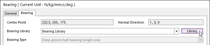
- Point: 232.5, 250, 175
- Direction: 1, 0, 0
After the Bearing dialog appears, click Library next to the Bearing Library.
After the Bearing Library dialog appears, adjust the values using the following information.
- Bearing Type: Deep groove ball bearing (single row)
- Diameter: (Inside) 85.000 mm
- Bearing: Timken 6317 (d=85.000 mm, D=180.000 mm, B=41.000 mm)
- Internal Clearance: C2
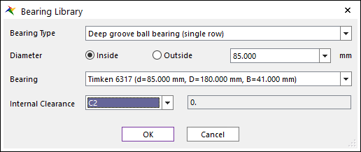
Click OK to close the Bearing Library dialog.
Click OK in the Bearing dialog to create BearingGroup1.
Delete the existing Bearing body where the BearingGroup1 has been created.
Repeat the Step 1~7 but change the Point value in the Step 2 as (-232.5, 250, 175).

9.4.4.3.2. To create the BearingGroup3, 4

Create the BearingGroup3, 4 using same method as above using the following information.

Point, Direction, WithDialog
- Point: (232.5, 250, -105), (-232.5, 250, -105)
- Direction: 1, 0, 0
Bearing Library
- Bearing Type: Deep groove ball bearing (single row)
- Diameter: (Inside) 65.000 mm
- Bearing: Timken 6313 (d=65.000 mm, D=140.000 mm, B=33.000 mm)
- Internal Clearance: C2

9.4.4.3.3. To create the BearingGroup5, 6

Create the BearingGroup5, 6 using same method as above using the following information.

Point, Direction, WithDialog
- Point: (232.5, 250, -325), (-232.5, 250, -325)
- Direction: 1, 0, 0
Bearing Library
- Bearing Type: Deep groove ball bearing (single row)
- Diameter: (Inside) 60.000 mm
- Bearing: Timken 6212 (d=60.000 mm, D=110.000 mm, B=22.000 mm)
- Internal Clearance: C2

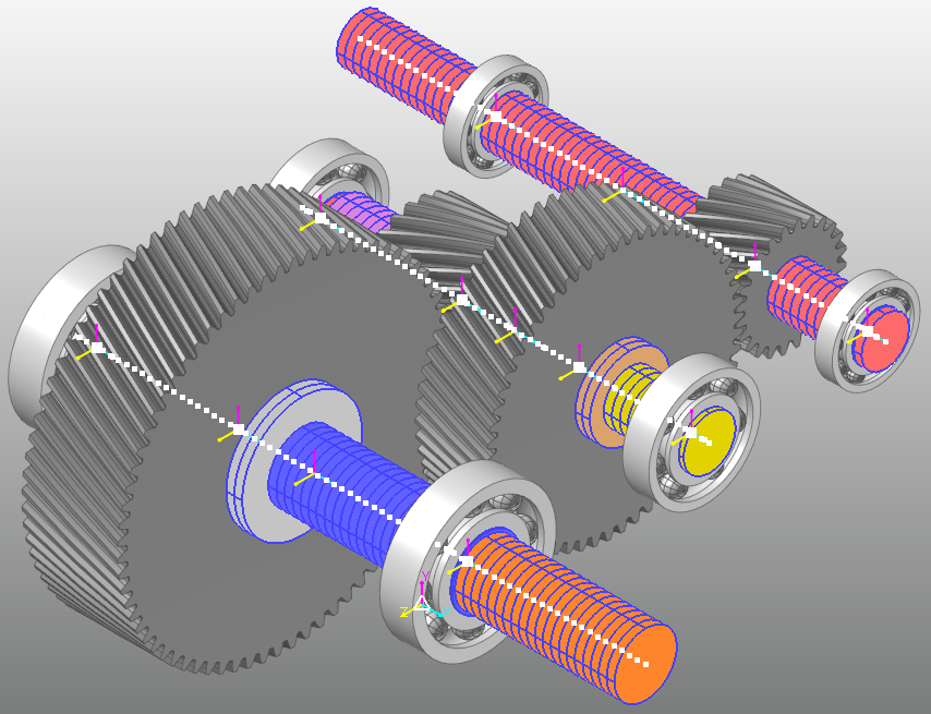
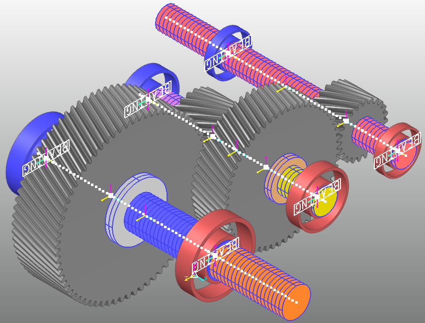
The model appears as shown in the figure below.

9.4.4.4. Saving the Model

Take a moment to save your model before you continue with the next chapter. (From File menu, click the Save function.)

9.4.5. Creating the Gear

9.4.5.1. Task Objective

In this chapter, you will create a Gear Pair using a KISSsoft Gear Train.

9.4.5.2. Estimated Time to Complete

15 minutes

9.4.5.3. Creating the Gear

You will create a KISSsoft Gear Train to analyze the dynamic behavior of a gear in a gearbox system.

9.4.5.3.1. To create a CylindricalGearGroup1

Delete the existing CAD Gear bodies.
From the KISSsoft group in the DriveTrain tab, click the GearTrain function.
Set the Creation Method to Point, Point, Direction, WithDialog and input the value using the following information.
- Point: -55, 250, 175
- Point: -55, 250, -105
- Direction: 1, 0, 0
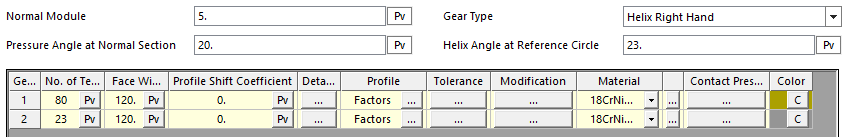
After the CylindricalGear dialog appears, input the values in the Gear Geometry section using the following information.
- Normal Module: 5
- Gear Type: Helix Right Hand
- Helix Angle at Reference Circle: 23
For rest of the parameters of Gear1, 2 input the values using following information. The dialog will appear as shown in the figure below.

Gear

No. of Teeth

Face Width

Profile Shift Coefficient

1

80

120

0

2

23

120

0
Click … in the Details of Gear1. Change the Inner Diameter value to 150 and click Close to exit the dialog. Change the Inner Diameter of Gear2 to 75 using above method.

Note

Tooth Tolerance

In the Tolerance dialog, you set the tolerances of tooth thickness, tip diameter and root diameter. If you set the Upper / Lower value as 0, it means no tolerance in gear shape. If you set the Upper / Lower values, KISSsoft automatically calculate the appropriate value between the upper and lower limit.

In Gear Pair section, change the Center Distance value to 280 and click Calc. in the Backlash to calculate backlash.

Note

Contact Analysis
In Contact Analysis dialog, the Number of Meshing Positions determines the number of calculation following the Path of Contact between a meshing teeth pair. The Number of Slices determines the number of axial cross sections of gear pair where the Meshing Position is calculated.
For example, if you set the Number of Meshing Position as 17 and 11 as the Number of Slices, the 17 meshing positions are distributed evenly throughout the path of contact in each one of 11 slices while the surface of gear tooth contacts the tooth surface of other gear.

Note

Difference between RecurDyn Gear Toolkit

The Gear Train dialog in DriveTrain Toolkit is created based on the KISSsoft User Interface. Some of the nomenclature is different from the RecurDyn Gear Toolkit. Below is the comparison of those parameters that has the same meaning but different names.

KISSsoft	RecurDyn
Normal Module	Module
Pressure Angle at Normal Section	Pressure Angle
Helix Angle at Reference Circle	Helix Angle
Face Width	Gear Width
Profile Shift Coefficient	Addendum Modification Coefficient
Inner Diameter	Hole Radius
Dedendum Coefficient	Dedendum Factor
Root Radius Coefficient	Hob Rack Radius Coefficient
Addendum Coefficient	Addendum Factor

Then, the CylindricalGear dialog appears as shown in the figure below.

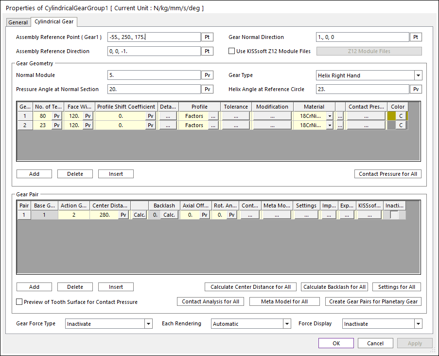
Click OK in CylindricalGear dialog to create CylindricalGearGroup1.

Note

Gear Modification

If you click Modification, you can create the various types of tooth modification. Profile/Tooth Modification has different input value regarding its type. For detailed information, refer to the manual.

(DriveTrain > Functions for DriveTrain > KISSsoft > Gear Train > Properties > Modification)

9.4.5.3.2. To create a CylindricalGearGroup2

Create the second Gear Pair using same method as above using following information.

Point, Point, Direction, WithDialog
- Point: 92, 250, -105
- Point: 92, 250, -325
- Direction: 1, 0, 0
Gear Geometry
- Normal Module: 5
- Gear Type: Helix Right Hand
- Helix Angle at Reference Circle: 23
Gear

No. of Teeth

Face Width

Profile Shift Coefficient

1

58

90

0

2

23

90

0
Inner Diameter
- Gear1: 100
- Gear2: 60
Change the Center Distance to 220 and click Calc. button of Backlash.

9.4.5.3.3. To adjust the Contact

In the Database, right-click the CylindricalGearGroup1 and click Properties in the Pop-up Menu.
In the Gear Pair section, Click … in the Meta Model.
Check the Import Meta Model File(*.gmm) and click ….
Open the GearBox_GearForce1.gmm file from directory below.
- <InstallDir>\Help\Tutorial\Toolkit\DriveTrain\GearBox
Close the Meta Model dialog.
Set the Gear Force Type to KISSsoft Force (Meta Model) as figure below.
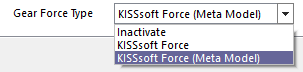
Click OK to close the dialog.
Repeat the Step 1~7 for the CylindricalGearGroup2 but changing the file to GearBox_GearForce2.gmm.

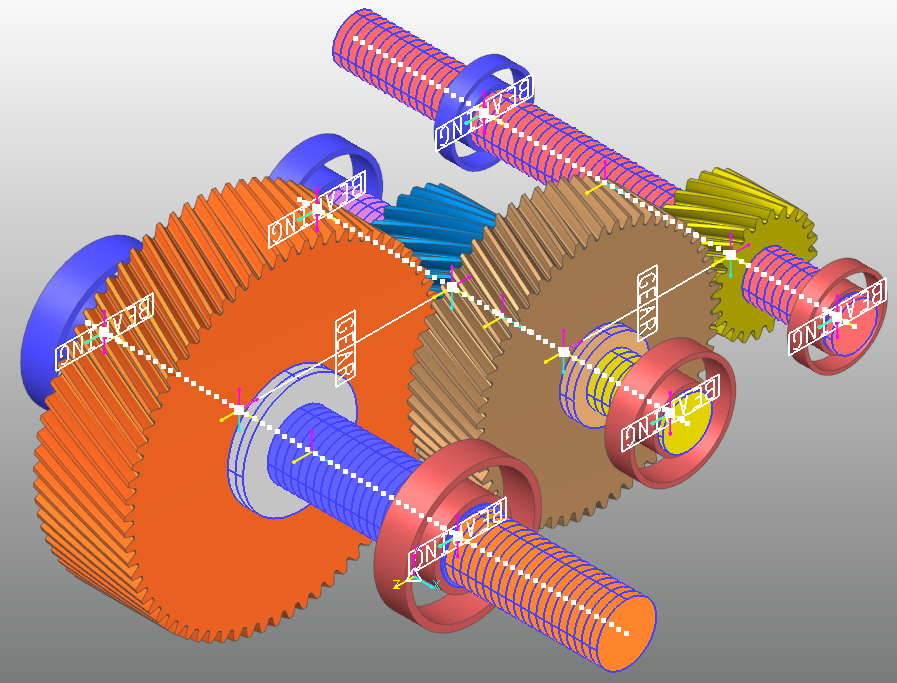
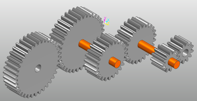
Then, model appears as shown in the figure below.

9.4.5.4. Saving the Model

Take a moment to save your model before you continue with the next chapter. (From File menu, click the Save function.)

9.4.6. Creating the Joint and Force

9.4.6.1. Task Objective

In this chapter, you will create the Joints and Forces.

Fixed Joint between Ground and Housing
Fixed Joint between Housing and Outer Bearing
Fixed Joint between Shaft and Inner Bearing
Revolute Joint between Ground and Shaft
Rotational Axial Force between Ground and Shaft

9.4.6.2. Estimated Time to Complete

20 minutes

9.4.6.3. Creating the Expression

You will create the expression which will be applied to Joints and Forces,

From the SubEntity tab, click the Expression function.
In the Expression List dialog, click Create.
In the Expression dialog, create the expression using the following information.

Name

Expression

Ex_Vel

STEP(TIME, 0, 0, 0.05, 2*PI*(10*TIME+1))

Ex_Torque

-STEP(TIME,0,0,0.05,10000)

9.4.6.4. Creating the Joint

9.4.6.4.1. To create the fixed joint

From the Joint group in the Professional tab, click the Fixed Joint function.
Set the Creation Method to Body, Body, Point and input the value using the following information.
- Body: Ground
- Body: LowerHousing
- Point: 245, -5, 485

Create the Fixed Joint between the Housing and Bodies using the following information.

Name	Body	Body	Point
Fixed1	Ground	LowerHousing	245, -5, 485
Fixed2	LowerHousing	UpperHousing	205, 250, 500
Fixed3	LowerHousing	BearingOuterBody1	232.5, 250, 175
Fixed4	LowerHousing	BearingOuterBody2	-232.5, 250, 175
Fixed5	LowerHousing	BearingOuterBody3	232.5, 250, -105
Fixed6	LowerHousing	BearingOuterBody4	-232.5, 250, -105
Fixed7	LowerHousing	BearingOuterBody5	232.5, 250, -325
Fixed8	LowerHousing	BearingOuterBody6	-232.5, 250, -325

Create the Fixed Joint between the Shaft and body using the following information.

Name	Body	Body	Point
Fixed9	Shaft1	BearingInnerBody1	232.5, 250, 175
Fixed10	Shaft1	CylindricalGear1	-55, 250, 175
Fixed11	Shaft1	BearingInnerBody2	-232.5, 250, 175
Fixed12	Shaft2	BearingInnerBody3	232.5, 250, -105
Fixed13	Shaft2	CylindricalGear2	-55, 250, -105
Fixed14	Shaft2	CylindricalGear3	92, 250, -105
Fixed15	Shaft2	BearingInnerBody4	-232.5, 250, -105
Fixed16	Shaft3	BearingInnerBody5	232.5, 250, -325
Fixed17	Shaft3	CylindricalGear4	92, 250, -325
Fixed18	Shaft3	BearingInnerBody6	-232.5, 250, -325

9.4.6.4.2. To create the revolute joint

You will create the Revolute Joint to set the motion in the gearbox.

From the Joint group in the Professional tab, click the Revolute Joint function.
Set the Creation Method to Body, Body, Point, Direction and input the value using following information.
- Body: Ground
- Body: Shaft3
- Point: -402, 250, -325
- Direction: 1, 0, 0
Create the Revolute Joint between the Shaft and Ground using the following information.

Name

Body

Body

Point

Direction

RevJoint1

Ground

Shaft3

-402, 250, -325

1, 0, 0

RevJoint2

Ground

Shaft1

455, 250, 175

1, 0, 0

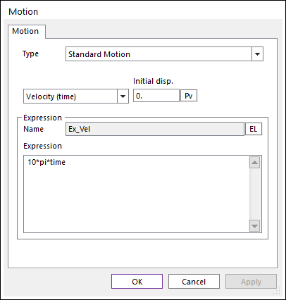
9.4.6.4.3. To adjust the motion

You will set the Motion in the RevJoint1.

In the Database Window, right-click the RevJoint1 and click Properties in the Pop-up menu.
Check the Include Motion and click Motion.
Change Displacement (time) to Velocity (time) and click EL.
Select Ex_Vel and click OK. The dialog appears as shown below.

9.4.6.5. Creating the Force

9.4.6.5.1. To create the rotational axial force

You will create the Rotational Axial Force to set the input torque of gearbox.

From the Force group in the Professional tab, click the Rotational Axial Force function.
Set the Creation Method to Joint.
Click RevJoint2 to create RotationalAxial1.

9.4.6.5.2. To create the rotational axial force

In the Database Window, right-click the RotationalAxial1 and click Properties in the Pop-up menu.
In the Rotational Axial Force page, click EL.
After Expression List dialog appears, select Ex_Torque by clicking it and click OK.
Click OK to close the dialog.

9.4.6.6. Performing Dynamic/Kinematic Analysis

In this section, you will run a dynamic/kinematic analysis to view the effect of forces and motion on the model you just created.

From the Simulation Type group in the Analysis tab, click the Dynamic / Kinematic function.
In the General page, define the end time of the simulation and number of steps:
- End Time: 2
- Step: 5000
- Plot Multiplier Step Factor: 2
Click Simulate. It will take approximately 3 minutes to complete the analysis. (CPU: Intel® Core™ i7-6700K CPU @ 4.00GHz)

9.4.7. Analyzing the Simulation Result

9.4.7.1. Task Objective

In this chapter, you will analyze the result of gearbox simulation.

9.4.7.2. Estimated Time to Complete

20 minutes

9.4.7.3. Analyzing the Shaft

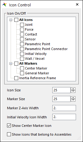
9.4.7.3.1. Adjust the icon control

In Render Toolbar, click the Icon Control tool as shown in the figure below.
Check Off the All Icons, All Markers, and Inertia Reference Frame as shown at below.

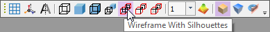
9.4.7.3.2. Adjust the rendering mode

In Render Toolbar, click the Wireframe with Silhouettes tool.

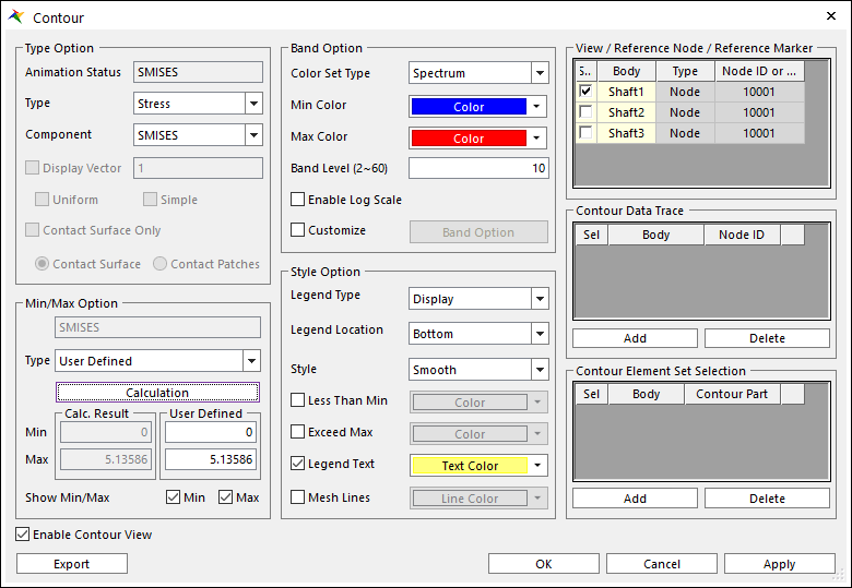
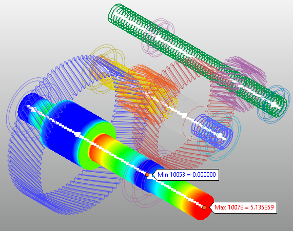
9.4.7.3.3. Adjust the contour

From the Shaft group in the DriveTrain tab, click the Contour function.
In the Contour Option group, change the Type as Stress and Component as SMISES.
In the Style Option group, change the Style from Stepped to Smooth.
In the right-side of the dialog, check off the Shaft2, Shaft3 in the View/Reference Node/Reference Marker.
Click Calculation, check the Show Min/Max option and click OK.

Then, the Contour dialog appears as shown in the figure below.

9.4.7.3.4. To play an animation

From the Animation Control group in the Analysis tab, click the Play function.

Then, maximum stress occurs in the Shaft1 after 9 frames.

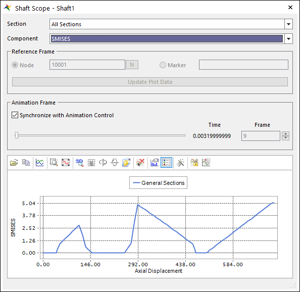
9.4.7.3.5. To view the shaft1 scope

From the Shaft group in the KISSsoft tab, click the Scope Control function.
After the Shaft Scope Control dialog appears, check Use option next to the Shaft1 and click Display.
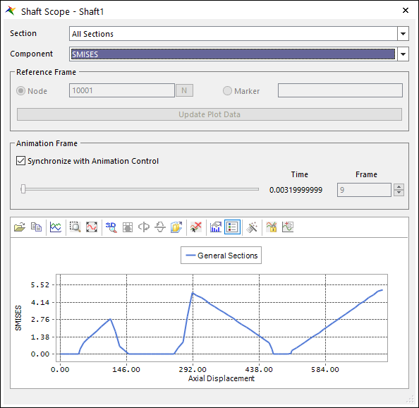
After the Shaft Scope - Shaft1 dialog appears, adjust the Component as SMISES.
Make sure the Synchronize with Animation Control option is checked in the Animation Frame section.
From the Animation Control group in the Analysis tab, click the Play function.

Then, you can see the changes of the SMISES of Shaft1 with Animation as shown in the figure below.

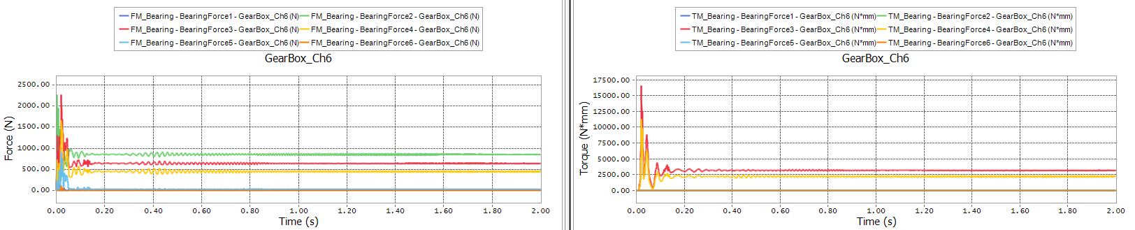
9.4.7.4. Analyzing the Bearing

From the Plot group in the Analysis tab, click the Plot Result function.
From the Windows group in the Home tab, click the Show All Windows function.
In the Plot Database Window, click the + button next to the Force.
Click the + button next to the DriveTrain_BearingForce.
Click the + button next to the BearingForce1.
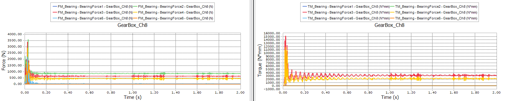
Click the upper-left pane of the Plot Window and double-click the FM_Bearing from the Plot Database Window.
Click the upper-right pane of the Plot Window and double-click the TM_Bearing from the Plot Database Window.
Repeat the Step 5~7 for the BearingForce2~6.

Then, Plot Window appears as shown in the figure below.

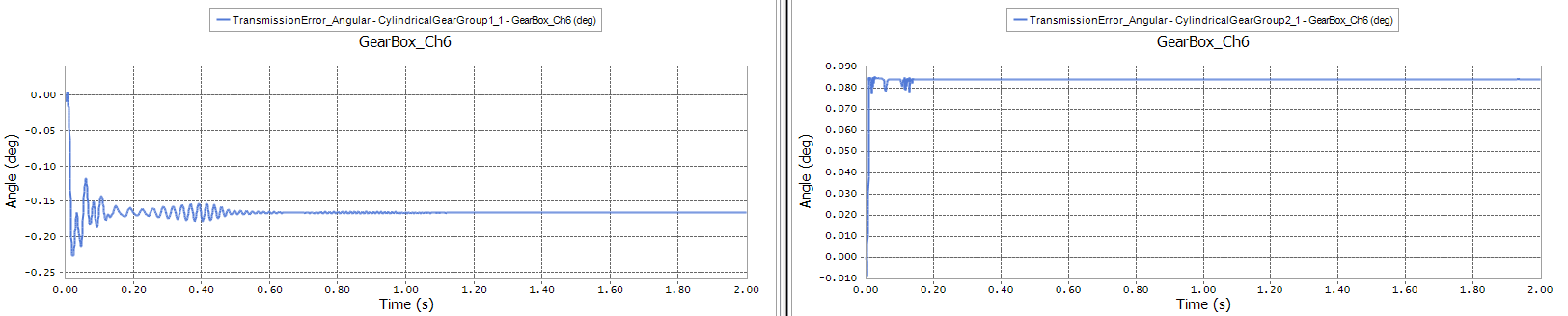
9.4.7.5. Analyzing the Gear

Click the + button next to the DriveTrain_GearForce.
Click the each + button next to the CylindricalGearGroup1_1 and CylindricalGearGroup2_1.
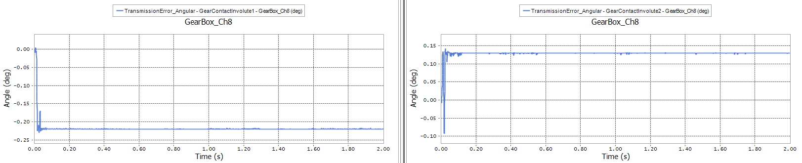
Click the lower-left pane of the Plot Window and double-click the TransmissionError_Angular from the CylindricalGearGroup1_1.
Click the lower-right pane of the Plot Window and double-click the TransmissionError_Angular from the CylindricalGearGroup2_1.

Then, Plot Window appears as shown in the figure below.

9.4.8. Involute Analytic Contact

9.4.8.1. Task Objective

In this chapter, you will learn how to use the Involute Analytic Contact.

9.4.8.2. Estimated Time to Complete

20 minutes

9.4.8.3. Creating the Involute Analytic Contact

Return to the GearBox model, you will learn how to use RecurDyn Involute Analytic Contact instead of KISSsoft Gear Contact.

9.4.8.3.1. Adjust the icon control

In Render Toolbar, click the Icon Control tool as shown in the figure below.
Check the Contact as shown at below.

9.4.8.3.2. Inactive the kisssoft gear contact

In the Database Window, right-click the CylindricalGearGroup1 and click Properties in the Pop-up menu.
Change the Gear force Type option to Inactivate at the bottom of Properties dialog.
Click OK to close the dialog.
Repeat the Step 1~3 for the CylindricalGearGroup2.

9.4.8.3.3. To create the involute analytic contact

From the Contact group in DriveTrain tab, click the Involute Analytic Contact function.
Set the Creation Method to KISSsoft body, KISSsoft body and select the CylindricalGear1 and CylindricalGear2.
Repeat the Step 1~2 for the CylindricalGear3, CylindricalGear4.

9.4.8.4. Performing Dynamic/Kinematic Analysis

In this section, you will run a dynamic/kinematic analysis to view the effect of Involute Analytic Contact on the model you just created.

From the Simulation Type group in the Analysis tab, click the Dynamic / Kinematic Analysis function.
Click Simulate.

9.4.8.5. Analyzing the Shaft

9.4.8.5.1. To view the shaft1 scope

From the Shaft group in the KISSsoft tab, click the Scope Control function.
After the Shaft Scope Control dialog appears, check Use option next to the Shaft1 and click Display.
After the Shaft Scope - Shaft1 dialog appears, adjust the Component as SMISES.
Make sure the Synchronize with Animation Control option is checked in the Animation Frame section.
From the Animation Control group in the Analysis tab, click the Play function.

Then, you can see the changes of the SMISES of Shaft1 with Animation as shown in the figure below.

The graph is almost same as the SMISES graph from Chapter 7.

9.4.8.6. Analyzing the Bearing

From the Plot group in the Analysis tab, click the Plot Result function.
From the Windows group in the Home tab, click the Show All Windows function.
In the Plot Database, click the + button next to the Force.
Click the + button next to the DriveTrain_BearingForce.
Click the + button next to the BearingForce1.
Click the upper-left pane of the Plot Window and double-click the FM_Bearing from the Plot Database Window.
Click the upper-right pane of the Plot Window and double-click the TM_Bearing from the Plot Database Window.
Repeat the Step 5~7 for the BearingForce2~6.

Then, Plot Window appears as shown in the figure below.

9.4.8.7. Analyzing the Gear

Click the + button next to the Contact.
Click the + button next to the Gear Involute Contact.
Click the each + button next to the GearContactInvolute1 and GearContactInvolute2.
Click the lower-left pane of the Plot Window and double-click the TransmissionError_Angular from the GearContactInvolute1.
Click the lower-right pane of the Plot Window and double-click the TransmissionError_Angular from the GearContactInvolute2.

Then, Plot Window appears as shown in the figure below.

9.4.9. Campbell Diagram

9.4.9.1. Task Objective

In this chapter, you will learn how to use the Campbell Diagram.

9.4.9.2. Estimated Time to Complete

20 minutes

9.4.9.3. Simulate the Campbell Diagram Model

You will open and simulate the already saved Campbell Diagram model.

9.4.9.3.1. To open the Campbell Diagram model

From the File menu, click the Open function.
From the Drivetrain tutorial directory, select the file Campbell_Diagram.rdyn.

(The file path: <InstallDir>\Help\Tutorial\Toolkit\Drivetrain\GearBox)
Click Open. The model appears as shown in the figure below.

9.4.9.3.2. To save the Campbell Diagram model

From the File menu, click the Save As function.
Save the model in different directory, because you cannot simulate in tutorial directory.

9.4.9.3.3. To simulate the Campbell Diagram model

You will run the Dynamic/Kinematic analysis because the model is already set.

From the Simulation Type group in the Analysis tab, click the Dynamic / Kinematic Analysis function.
Click Simulate. It will take approximately 30 seconds to complete the analysis. (CPU: Intel® Core™ i7-6700K CPU @ 4.00GHz)

9.4.9.4. Adjusting the Analysis Tab

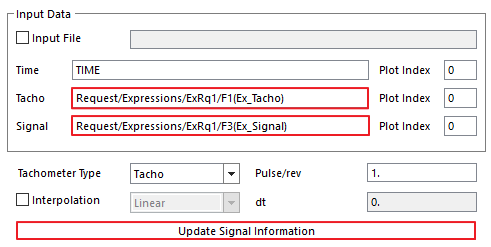
9.4.9.4.1. To adjust the Input Data

From the Plot group in the Analysis tab, click the Plot Result function.
From Tool tab, click the Campbell (3D) function.
In Plot Database Window, expand the Request -> Expression -> ExRq1.
Drag & Drop the F1(Ex_Tacho) in the Tacho from Input Data.
Drag & Drop the F3(Ex_Signal) in the Signal from Input Data.
Click Update Signal Information to update the below parameters.

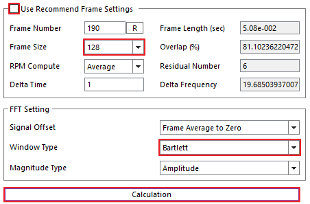
9.4.9.4.2. To adjust the Frame Settings

Check off the Use Recommended Frame Settings.
Change Frame Size to 128.
Change Window Type to Bartlett.
Click Calculation.

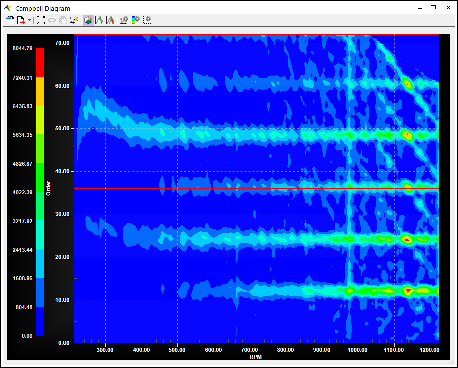
9.4.9.5. Adjusting the Plot Tab

From Campbell Diagram dialog, click Plot page.
Change Graph Type to Color Map (2D).
Change Graph Option to RPM-Order.
Check Draw Order Line.
Adjust the Order Line parameters using the following information.
- Minimum Order: 0
- Maximum Order: 72
- Gap: 12
- Resolution: 100
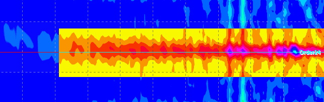
In the below-part of the dialog, click Plot to open the graph. The graph will be shown as below.

9.4.9.6. Adjusting the Campbell Diagram

9.4.9.6.1. To use Zoom

Drag as below figure to include Order 24.
The selected part is Zoomed.
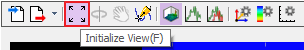
From Toolbar, click Initialize View to initialize the view.

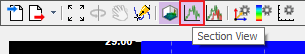
9.4.9.6.2. To use Section View

From Toolbar, click Section View.
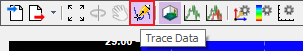
At the left-side of the Section View, click Trace Data.
To set the Section, left click in the graph where X, Y is (1134, 24).
Right-click in the Y-Section as shown in the figure below and click Add to Plot in the Pop-up menu.
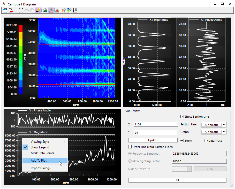
Y-Section Data is drawn in the Plot.

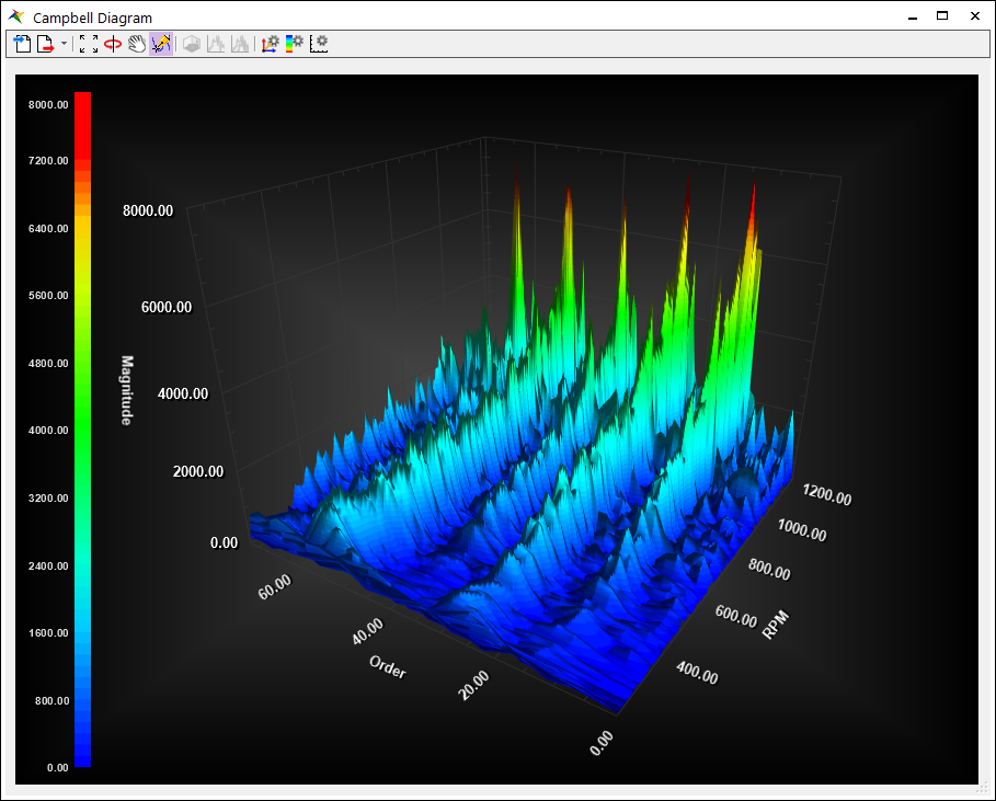
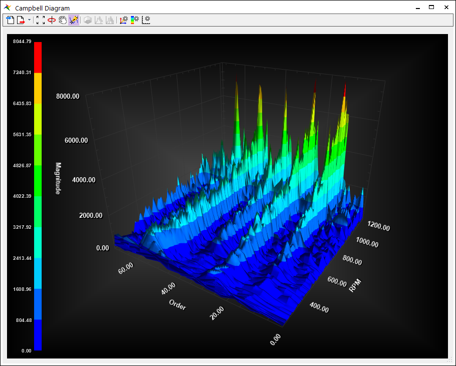
9.4.9.6.3. To use 3D plot

Close the Graph and go back to the Campbell Diagram dialog.
In the Plot page, change the Graph Type to Surface Contour (3D).
Click Plot in the below-part of the dialog. 3D Plot will be shown as figure below.

Note

Mouse Operation
Rotate View: Dragging with left click will rotate the view.
Translate View: Dragging with left click while pressing Shift key will rotate the view.
Light Change: Dragging with middle click (mouse scroll button) will change the location of the light source.

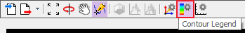
9.4.9.6.4. To adjust the Contour

In the Toolbar, click Contour Legend.
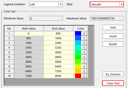
Change Style to Smooth.
In the Color Set section, click Color Tool.
In the Color Tool dialog, change Max Value to 8000, click Update and OK.
Contour Legend dialog will be shown as below.
Click OK to apply the changes. The graph will be shown as below.

Section	L	Ro	Ri	Element Size
1	120	42.5	0	10
2	160	75	0	10
3	230	42.5	0	10
4	200	39	0	10

No	Center Position	Width	Type
1	22.5	41	RBE2
2	200	120	RBE2
3	487.5	41	RBE2

Section	L	Ro	Ri	Element Size
1	50	32.5	0	10
2	235	37.5	0	10
3	125	50	0	10
4	100	32.5	0	10

No	Center Position	Width	Type
1	22.5	33	RBE2
2	200	120	RBE2
3	347	90	RBE2
4	487.5	33	RBE2