5.1. Pendulum Tutorial (FMPY)

5.1.1. Getting Started

5.1.1.1. Objective

In this tutorial, we will cover how to perform and control analysis of dynamic system using Python script. We will set up inputs and outputs in RecurDyn using FMI method and co-simulation Python using FMPY and TensorFlow modules.

This system analysis the inverted pendulum that can move left and right. Describes the process of implementing a control system so that the pendulum is balanced in an upright position (Target) through a force acting on the base.

5.1.1.2. Prerequisites

Basic physics knowledge is required and an understanding of system input and output is required. And it requires basic knowledge of Python.

5.1.1.3. Procedures

This tutorial consists of the following chapters. The time required to complete each chapter is shown in the table below.

Procedures	Time (minutes)
Setting Input and Output of Control System	5
Installing Python and Module	20
PID Control Using FMI (RecurDyn Client)	20
NN Control Using FMI (RecurDyn Client)	120
Total	165

5.1.1.4. Estimated Time to Complete

165 minutes

5.1.2. Setting Input and Output of Control System

5.1.2.1. Task Objective

This chapter learns how to set up the Inputs and Outputs of a mechanical model to the control system.

5.1.2.2. Estimated Time to Complete

5 minutes

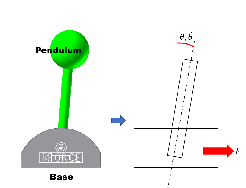
5.1.2.3. Understanding the System

Before setting up the inputs and outputs, please refer to the figure below to help you understand the mechanical system.

A note about the model.

• Offset by 5 degrees so that the pendulum can be moved by gravity.

• Pendulum is connected to the base by a revolute joint. Base is connected to ground by translational joint and translational force.

• As shown in the figure on the below, it can be seen that the component of the force input to the translational force affect \(\theta\) and \(\dot{\theta }\). Therefore, it can be seen that the input component of the control system is the translational force and the output component is the angle and angular velocity of the pendulum.

• The model analysis 5 seconds.

5.1.2.4. Starting RecurDyn and Opening the Model

5.1.2.4.1. To start RecurDyn:

1. Double-click the RecurDyn icon on the desktop.

2. In the Start RecurDyn dialog, click x to close it.

5.1.2.4.2. To open the Model:

1. Choose Open from the File menu.

2. Open the RecurDyn model that has completed basic joint and force modeling.

   (The file path: <InstallDir>\Help\Tutorial\Control\FMPY\Pendulum_Tutorial_Start.rdyn)

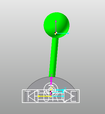
3. Confirm the model is open.

   

5.1.2.5. Creating General Plant Input

Generates a General Plant Input to receive forces input from an external program (FMPY).

5.1.2.5.1. Create General Plant Input

1. On the Communicator tab, in the GPlant In/Out group, Click the General Plant Input function.

2. Click Add in the General Plant Input List dialog to create GPlantInput1.

   

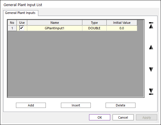
3. Click OK to close the General Plant Input List dialog.

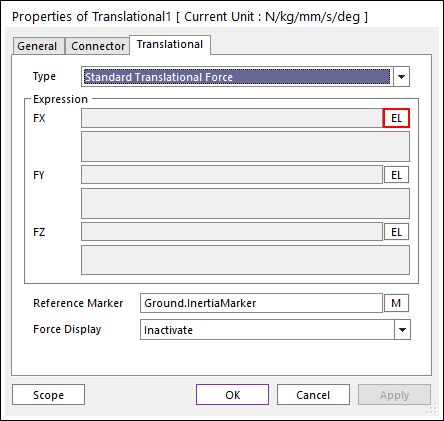
4. In the Database Window, select Translational1 of force entity, right-click and click properties.

5. Click EL of the FX of Expression to open the Expression List dialog and click Create.

   

6. Enter Ex_GPIN_Force as the Expression Name.

7. Enter GPIN(1) in the expression.

8. Click Add in the Argument List.

9. Drag & drop GPlantInput1 from the Database Window to ID 1 of the Argument List as shown in the figure.

   

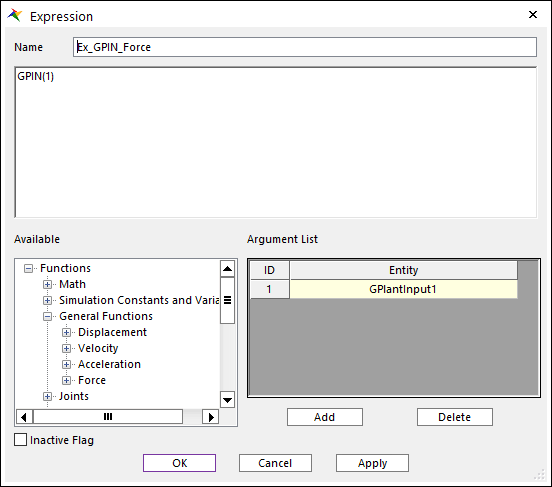
10. Click OK to complete the Expression setting.

11. Click OK in the Expression List dialog to close.

12. Click OK in the Translational1 property dialog to complete the expression setting.

5.1.2.6. Creating General Plant Output

Create a General Plant Output to pass the angle and angular velocity of the Pendulum to Python.

5.1.2.6.1. Create General Plant Output

1. On the Communicator tab, in the Control group, click the General Plant Output function.

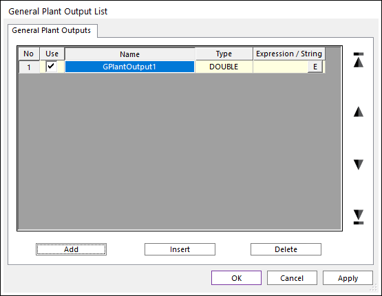
2. In the General Plant Output List dialog, click Add.

3. When GPlantOutput1 is created, click E in Expression/String.

   

4. In the Expression List dialog, click Create.

5. Change the Name of Expression to Exp_GPlantOutput1.

6. In the expression, enter the function PSI(1,2).

7. In the Argument List, click Add to create two IDs.

8. Enter the following markers in the Argument List.

   • ID 1 : Pendulum.Marker1

   • ID 2 : Base.Marker1

   

9. Click OK to complete creating the expression.

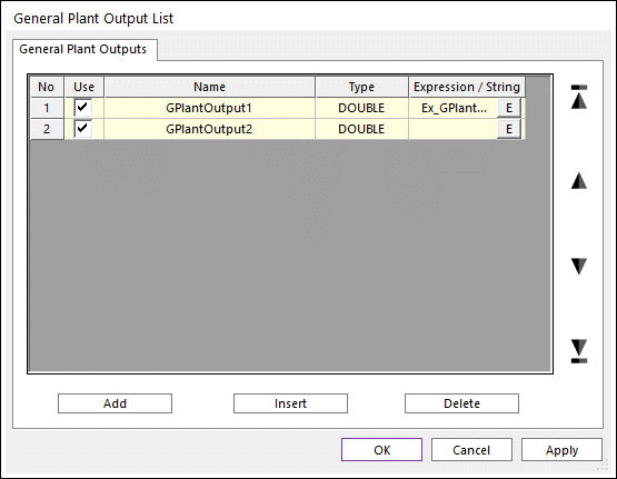
10. In the General Plant Output List dialog, Click Add.

11. When GPlantOutput2 is created, click E in Expression/String.

    

12. In the Expression List dialog, click Create.

13. Change the Name of Expression to Exp_GPlantOutput2.

14. Enter the function WZ(1,2) in the Expression.

15. In the Argument List, click Add to create two IDs.

16. Enter the following markers in the Argument List.

    • ID 1 : Pendulum.Marker1

    • ID 2 : Base.Marker1

    

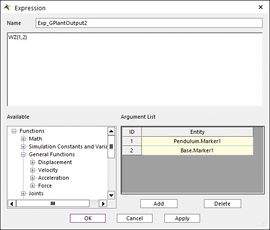
17. Click OK to complete creating the expression.

18. Save the finished model as Pendulum_Plant_Model.rdyn.

19. Close the model.

5.1.3. Installing Python and Module

5.1.3.1. Objective

In this chapter, we explain the installation of Python to be co-simulated with RecurDyn and setting of modules required for the tutorial using Windows Batch Command and PyCharm.

5.1.3.2. Estimated Time to Complete

20 minutes

5.1.3.3. Installing Python and PyCharm

Describes installing Python and PyCharm to run FMPY.

5.1.3.3.1. To Install Python

1. Access the website. (http://www.python.org/downloads/)

2. In Release, select your Python version. The modules used in this tutorial use TensorFlow and FMPY. Two modules required Python 3.5 or higher version, so you need to install Python that meets the conditions.

   (The Python version used in this tutorial is version 3.9)

   

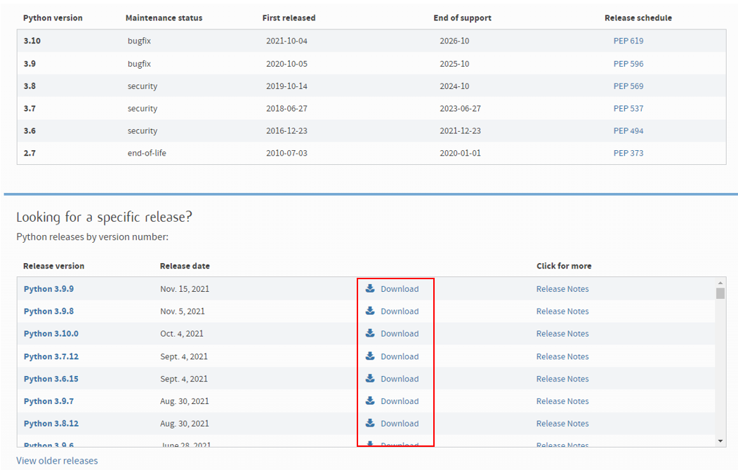
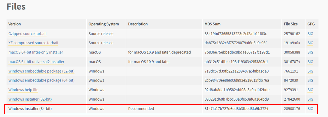
3. On the page that appears by selecting a version, select Windows installer(64-bit) in the Files area to install.

   

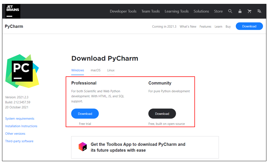
5.1.3.3.2. To Install Pycharm

1. Access the website. (http://www.jetbrains.com/pycharm/download/)

2. It is suitable for the OS of the PC user is using and installs it by selecting Professional or Community according to the policy.

   

5.1.3.4. Installing Python Module

It explains how to install Python FMPY and TensorFlow modules required to proceed with the tutorial. This tutorial explains how to install using two programs, Windows Batch Command and PyCharm

5.1.3.4.1. To Install Python Module in Window Batch Command

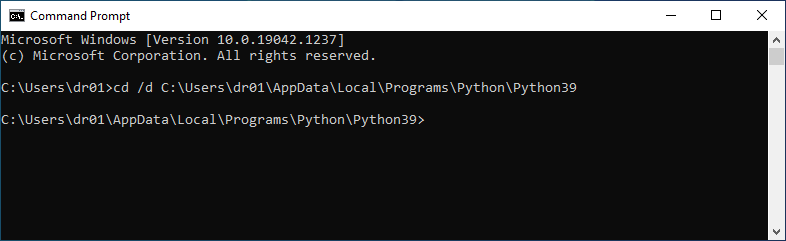
1. Run Windows Batch Command (CMD.exe).

2. [cd /d <Python Install Directory>] Use the command to navigate to the Python installation path.

   (The default installation path is C:\Users\[UserName]\Appdata\Local\Programs\Python\Python39 . In this case, you need to run CMD.exe with administrator privileges.)

   

3. [python -m pip install fmpy] Install FMPY in Python using this command.

   

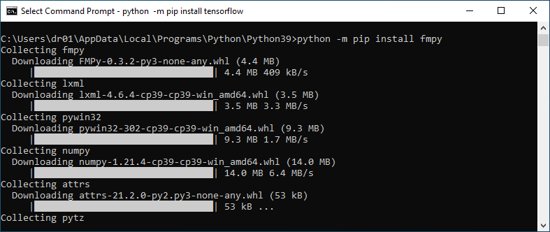
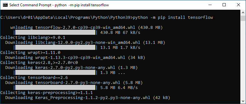
4. [python -m pip install tensorflow] Install TensorFlow in Python using this command.

   

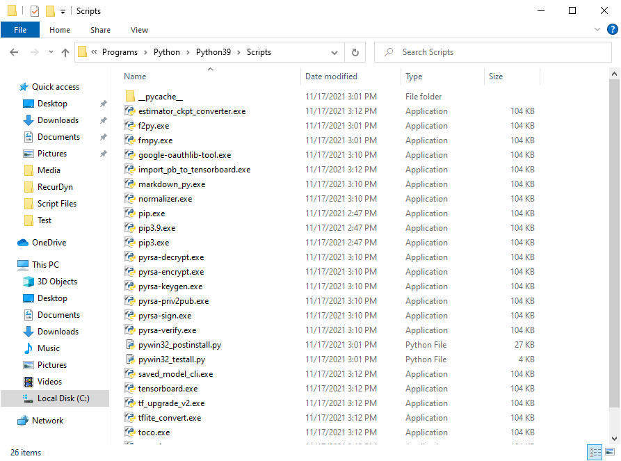
5. Check in [<Python Install Directory>\Scripts] that the installation is complete.

   

5.1.3.4.2. To install Python Module in PyCharm

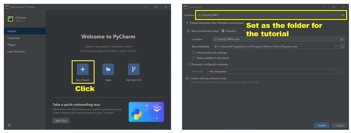
1. Run PyCharm.

2. Create a project in the tutorial folder.

   

3. Click File > Settings on the ribbon menu in the created project.

   

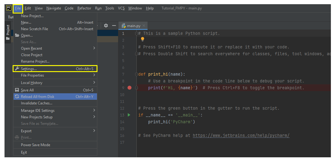
4. Click the + button in the Python Interpreter and search for fmpy in the Available Package dialog. Click the Install Package button to install the relevant package.

   

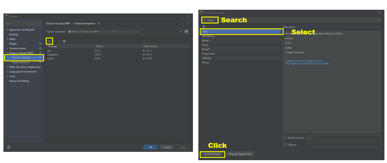
5. In the same way, in the Available Package dialog, search for TensorFlow in the search tab and install it.

5.1.4. PID Control Using FMI (RecurDyn Client)

5.1.4.1. Objective

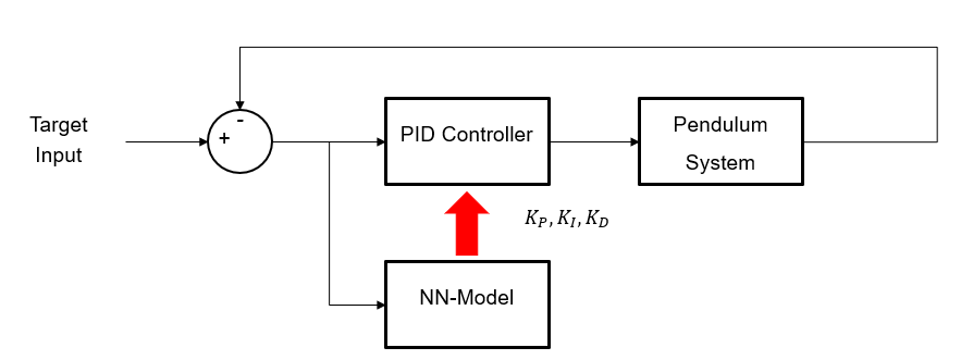
RecurDyn and FMPY are Co-Simulated using FMI method. To prevent the pendulum from falling over, it uses the error between the target value and the current angle and angular velocity to transmit the force to the base through PID control.

In this chapter, we aim to implement the control system when Python is the host program and RecurDyn is the client program. Here, host is the main program, which means that the client program RecurDyn is analysis by executing the code written in Python.

5.1.4.2. Estimated Time to Complete

20 minutes

5.1.4.3. Exporting *.fmu File from RecurDyn Model

Obtain the *.fmu file require for Co-Simulation from the RecurDyn model.

5.1.4.3.1. To Open the Model

1. Run the Pendulum_Plant_Model.rdyn model created in Chapter 2.

2. Save it as Pendulum_PID_FMPY_Client.rdyn.

5.1.4.3.2. Setting up RecurDyn FMI Co-Simulation Environment

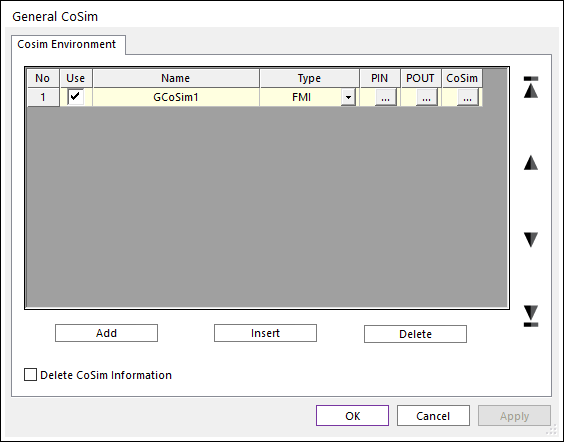
1. On the Communicator tab in Control group, Click the General CoSim function.

2. On the CoSim Environment page of the General CoSim dialog, click Add.

   

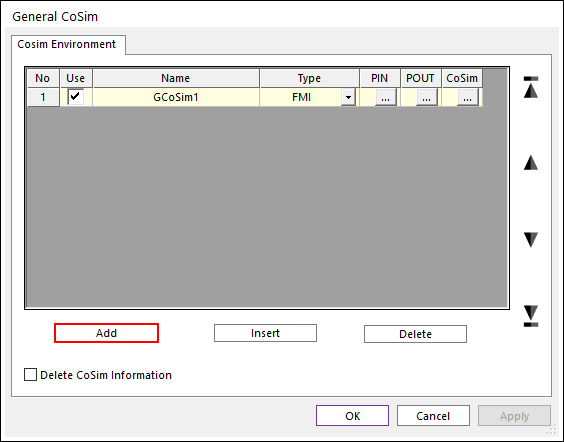
3. Set Name to GCoSim1.

4. Select Type as FMI.

5. Click … in PIN.

6. Click Add in the General Plant Input List (GCoSim1) dialog to add GPlantInput1.

   

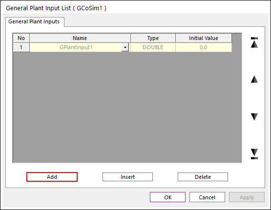
7. Click OK.

8. On the CoSim Environment page of the General CoSim dialog, click … of POUT.

   

9. In the General Plant Output List (GCoSim1) dialog, double-click the Add button to add 2 GPlantOutputs.

   

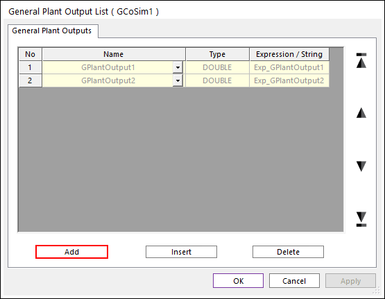
10. Click OK.

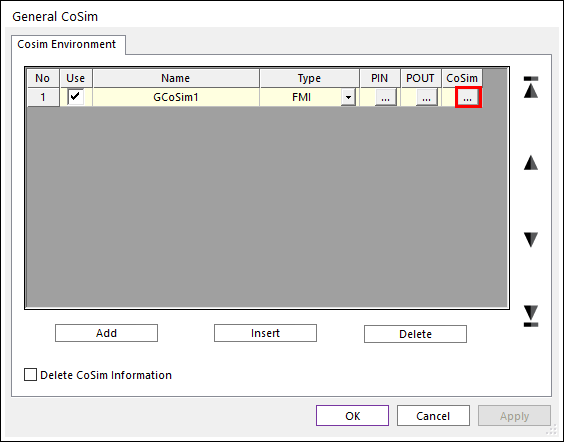
11. On the CoSim Environment page of the General CoSim dialog, click … for CoSim.

    

12. On the FMI (GCoSim1) dialog CoSim Environment page, select the Export option.

13. Select Interface Version as 2.0.

14. Enter Pendulum_PID_FMPY_Client in the Create a FMU File window, click Export, and check whether the fmu file is created in the folder.

    

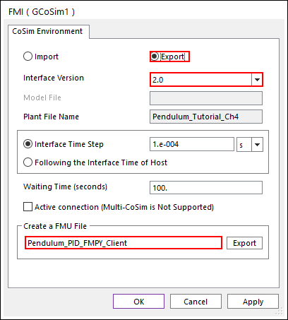
15. Click OK in the FMI (GCoSim1) dialog to complete the setting.

16. On the CoSim Environment page of the General CoSim dialog, click OK to complete the settings.

17. Save the model again and exit RecurDyn.

5.1.4.4. Running the Python(*.py) File to Proceed with Co-Simulation

In this section we explain how to write a script that calls FMPY in Python to perform PID Control and executes it to perform Co-Simulation. For Python files, use the files provide in the tutorial.

5.1.4.4.1. To Copy *.py file

• Copy the python file for PID control in the path below to a folder in the path to run simulation.

  (The file path: <InstallDir>\Help\Tutorial\Control\FMPY\FMPY_PID_Control.py)

5.1.4.4.2. Python File Description and Modification

Proceed explanation of the copied python file.

from fmpy import read_model_description, extract
from fmpy.fmi2 import FMU2Slave
import numpy as np

Load the fmpy module and load the functions to use in that module.

# define the fmu file name
fmu_filename = 'C:\\Tutorial_FMPY\\Pendulum_PID_FMPY_Client.fmu'

Enter the full path to the name of the *.fmu file create earlier in the RecurDyn model.

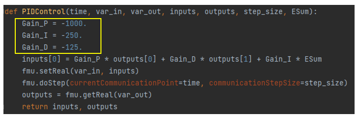
def PIDControl(time, var_in, var_out, inputs, outputs, step_size, ESum):
    Gain_P = -1000.
    Gain_I = -250.
    Gain_D = -125.
    inputs[0] = Gain_P \* outputs[0] + Gain_D \* outputs[1] + Gain_I \* ESum fmu.setReal(var_in, inputs)
    fmu.doStep(currentCommunicationPoint=time, communicationStepSize=step_size)
    outputs = fmu.getReal(var_out)
    return inputs, outputs

Defines a function to use for PID control. The components input to the inputs of the above function are the same as the formula for PID control for each time step.

inputs = \(Error={{K}_{P}}\cdot e(t)+{{K}_{i}}\int{e(t)dt}+{{K}_{i}}\cdot \frac{d}{dt}e(t)\) fmu.setReal is a function that input to RecurDyn, a client program, and fmu.doStep is a function that moves from the current itme to the next step. And get the RecurDyn output from the next step with fmu.getReal.

# read the model description
model_description = read_model_description(fmu_filename)

# Initialize analysis parameter
var_input = {}
var_output = {}
start_time = 0.0
stop_time = 0.0
step_size = 0.0
ninput = 0
noutput = 0
ESum = 0

Read the fmu file in the specified path using Read_model_description function and declares the necessary parameters.

for variable in model_description.modelVariables:
    if "RD_StopTimeDefined" in variable.name:
        stop_time = float(variable.start)
        stop_time = stop_time
    if "InterfaceStepSize" in variable.name:
        step_size = float(variable.start)
    if "nPinput" in variable.name:
        ninput = int(variable.start)
    if "nPoutput" in variable.name:
        noutput = int(variable.start)
    if "Input Data1 of Plant(RD)" in variable.description:
        var_input[variable.name] = variable.valueReference
    if "Output Data1 of Plant(RD)" in variable.description:
        var_output[variable.name] = variable.valueReference

Read the fmu file and set the model variable.

# IO variable reference to list
var_in = list(var_input.values())
var_out = list(var_output.values())
# extract the FMU
unzipdir = extract(fmu_filename)
fmu = FMU2Slave(guid=model_description.guid, unzipDirectory=unzipdir,
modelIdentifier=model_description.coSimulation.modelIdentifier, instanceName='instance1')

Unzip the fmu file.

# initialize
fmu.instantiate()
fmu.setupExperiment(startTime=start_time, stopTime = stop_time)
fmu.enterInitializationMode()
fmu.exitInitializationMode()

# simulation standby
time = start_time states = [[0 for \_ in range(len(var_in) + len(var_out) + 1)]]**

# states = np.zeros(len(var_in) + len(var_out))
outputs = [0 for \_ in range(len(var_out))]

# simulation loop
while time <= (stop_time+1):
   inputs = np.zeros(len(var_in)).tolist()
   inputs, outputs = PIDControl(time, var_in, var_out, inputs, outputs, step_size, ESum)
   ESum += outputs[0] \* step_size states.append(([time] + inputs + outputs))
   time += step_size

# Simulation Terminate
fmu.terminate()
fmu.freeInstance()

Run analysis.

5.1.4.4.3. Running Python File with Windows Batch Command (PD Control)

You can proceed with PD Control by changing the Gain_I value of the PIDControl function to 0 in the FMPY_PID_Control.py file above. And describes how to run the modified *.py file with Windows Batch Command.

def PIDControl(time, var_in, var_out, inputs, outputs, step_size, ESum):
    Gain_P = -1000.
    Gain_I = 0.
    Gain_D = -125.

1. Run Windows Batch Command (CMD.exe).

2. Enter the following command to move the folder where the *.py file is located.

   [Command: cd /d “<Path located py file>”]

3. Run the python file with the following command.

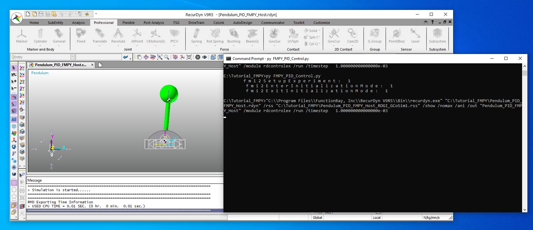
   [Command: py FMPY_PID_Control.py]

4. You can see the analysis in progress.

   

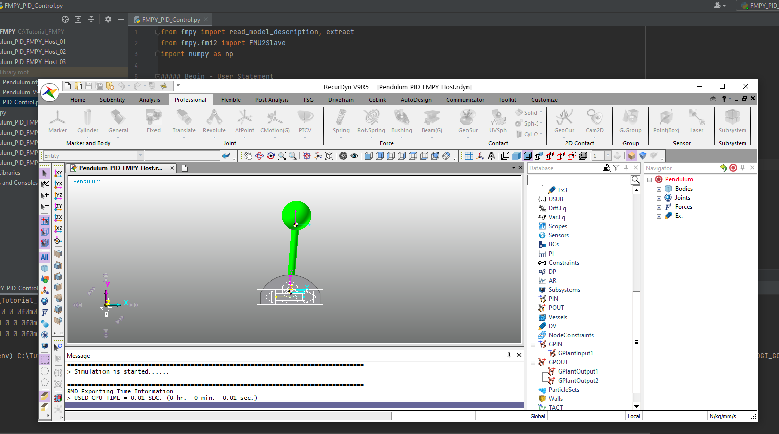
5.1.4.4.4. Check the Results

1. Run RecurDyn.

2. Create a new model and click the Plot Result function in the Plot group of the Analysis tab.

3. Load the analysis result file (Pendulum_PID_FMPY_Host.rplt).

4. On the Home tab of the Plot, select the Show Upper Windows function.

5. In the Plot Database Window, draw GPlantOutput1 of GPlant Output on the left and GPlantOutput2 on the right.

   

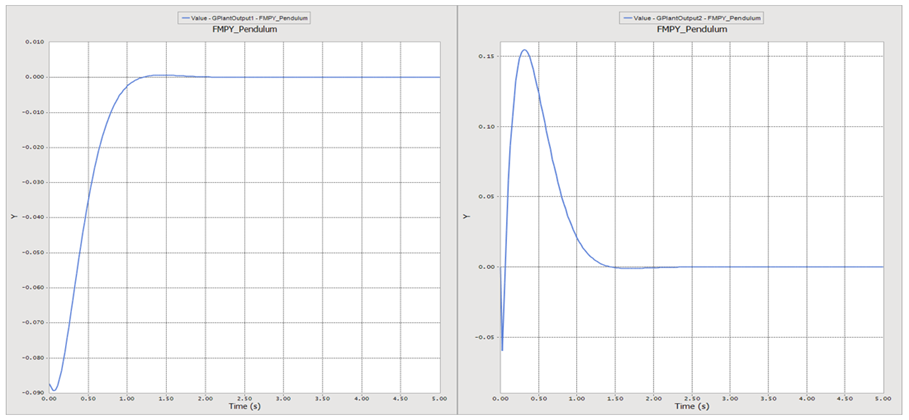
6. You can see that the analysis is in progress by applying the gain value of the controller.

5.1.4.4.5. Running Python File with PyCharm (PID Control)

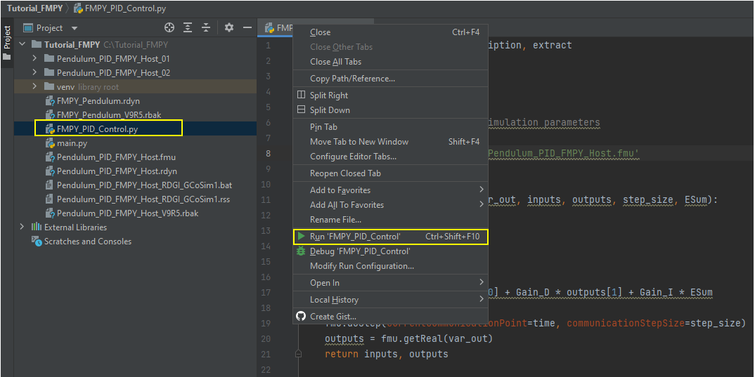
1. Run Pycharm.

2. Open the *.py file in project. After open, you can proceed with PID control by setting the Gain_P, Gain_I, and Gain_D values of the PIDControl function as follows.

   

3. Click the Run button to run the python file or use the right-click button on the project name to run the python file.

   

4. You can see the analysis in progress.

   

5.1.4.4.6. Check the Results

1. Run RecurDyn.

2. Create a new model and click the Plot Result function in the Plot group of the Analysis tab.

3. Load the analysis result file (Pendulum_PID_FMPY_Host.rplt).

4. On the Home tab of the Plot, select the Show Upper Windows function.

5. In the Plot database, draw GPlantOutput1 of GPlant Output on the left and GPlantOutput2 on the right.

   

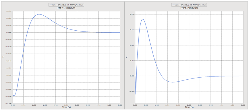
6. You can see that the analysis is in progress by applying the gain value of the controller.

5.1.5. NN Control Using FMI (RecurDyn Client)

5.1.5.1. Objective

Using RecurDyn, FMPY, and TensorFlow, we build a control system that improves PID control in the form of a compensator for PID controller. RecurDyn and Host program basically communicate using FMPY, and by using TensorFlow for advanced PID control, the result value obtained through PID control is corrected to build a system that reaches the target value more quickly and stably. Each of the initial PID values used and compared in the corresponding chapter is P=-1000, I=0, D=-215, which confirms how much efficiency can be shown from PD Control.

Please note that the overall analysis time takes longer than the existing PID control because NN control progresses learning step by step.

5.1.5.2. Estimated Time to Complete

120 minutes

5.1.5.3. Exporting *.fmu File from RecurDyn Model

Obtain the *.fmu file require for Co-Simulation from the RecurDyn model.

5.1.5.3.1. To Open the Model

1. Run the Pendulum_Plant_Model.rdyn model created in Chapter 2.

2. Save it as Pendulum_PID_FMPY_Client.rdyn .

5.1.5.3.2. Setting up RecurDyn FMI Co-Simulation Environment

1. On the Communicator tab in Control group, Click the General CoSim function.

2. On the CoSim Environment page of the General CoSim dialog, click Add.

   

3. Set Name to GCoSim1.

4. Select Type as FMI.

5. Click … in PIN.

6. Click Add in the General Plant Input List (GCoSim1) dialog to add GPlantInput1.

   

7. Click OK.

8. On the CoSim Environment page of the General CoSim dialog, click … of POUT.

   

9. In the General Plant Output List (GCoSim1) dialog, double-click the Add button to add 2 GPlantOutputs.

   

10. Click OK.

11. On the CoSim Environment page of the General CoSim dialog, click … for CoSim.

    

12. On the FMI (GCoSim1) dialog CoSim Environment page, select the Export option.

13. Select Interface Version as 2.0.

14. Enter Pendulum_NNControl_Client in the Create a FMU File window, click Export, and check whether the fmu file is created in the folder.

    

15. Click OK in the FMI (GCoSim1) dialog to complete the setting.

16. On the CoSim Environment page of the General CoSim dialog, click OK to complete the settings.

17. Save the model again and exit RecurDyn.

5.1.5.4. Running the Python(*.py) File to Proceed with Co-Simulation

Explain how to write a script that calls FMPY and TensorFlow in Python to perform NN control and run it to perform Co-Simulation. For Python files, use the files provided in the tutorial.

5.1.5.4.1. To Copy *.py file

• Copy the python file for NN control in the path below to a folder in the path to run.

  (The file path: <InstallDir>\Help\Tutorial\Control\FMPY\FMPY_NN_Control.py)

5.1.5.4.2. Python file description and modification

Proceed with the explanation of the copied python file.

import random
import numpy
from fmpy import read_model_description, extract
from fmpy.fmi2 import FMU2Slave
import numpy as np
import os os.environ['TF_CPP_MIN_LOG_LEVEL'] = '2'
import tensorflow as tf from tensorflow
import keras from tensorflow.keras
import layers from tensorflow.keras
import models from tensorflow.keras
import losses from keras.models
import Sequential
import numpy as np

Load the fmpy module and the Keras TensorFlow module, and load the function using in those modules.

# define the fmu file name
fmu_filename = 'C:\Tutorial_FMPY\Pendulum_NNControl_Client.fmu'

Enter the full path to the name of the *.fmu file created earlier in the RecurDyn model.

def PIDControl(time, var_in, var_out, inputs, outputs, step_size, ESum, Gain_P, Gain_D, Gain_I):
    ESum += outputs[0]*step_size
    inputs[0] = Gain_P \* outputs[0] + Gain_D \* outputs[1] + Gain_I \* ESum
    fmu.setReal(var_in, inputs)
    fmu.doStep(currentCommunicationPoint=time, communicationStepSize=step_size)
    outputs = fmu.getReal(var_out)
    return inputs, outputs**

Defines a function to use for PID control. The components input to the inputs of the above function are the same as the formula for PID control for each time step.

inputs = \(Error={{K}_{P}}\cdot e(t)+{{K}_{i}}\int{e(t)dt}+{{K}_{i}}\cdot \frac{d}{dt}e(t)\) The difference from the previous code is that P, I, and D values are updated at every step, so P, I, D gain values are added as arguments of the function.

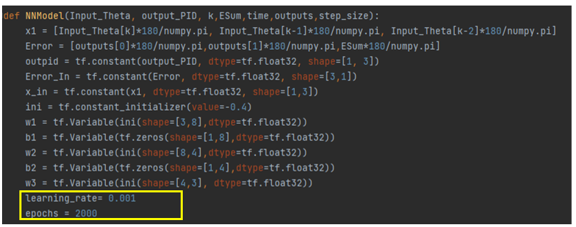
def NNModel(Input_Theta, output_PID, k,ESum,time,outputs,step_size):
    x1 = [Input_Theta[k]*180/numpy.pi, Input_Theta[k-1]*180/numpy.pi, Input_Theta[k-2]*180/numpy.pi]
    Error = [outputs[0]*180/numpy.pi,outputs[1]*180/numpy.pi,ESum*180/numpy.pi]
    outpid = tf.constant(output_PID, dtype=tf.float32, shape=[1, 3])
    Error_In = tf.constant(Error, dtype=tf.float32, shape=[3,1])
    x_in = tf.constant(x1, dtype=tf.float32, shape=[1,3])
    ini = tf.constant_initializer(value=-0.4)
    w1 = tf.Variable(ini(shape=[3,8],dtype=tf.float32))
    b1 = tf.Variable(tf.zeros(shape=[1,8],dtype=tf.float32))
    w2 = tf.Variable(ini(shape=[8,4],dtype=tf.float32))
    b2 = tf.Variable(tf.zeros(shape=[1,4],dtype=tf.float32))
    w3 = tf.Variable(ini(shape=[4,3], dtype=tf.float32))
    learning_rate= 0.01
    epochs = 500
    l=0
    for epoch in range(0,epochs):
        with tf.GradientTape() as t:
            t.watch(x_in)
            h1 = tf.matmul(x_in, w1)
            h2 = tf.matmul(h1, w2)
            h3 = tf.matmul(h2, w3)
            test = tf.matmul(outpid,Error_In) - tf.matmul(h3,Error_In)
            loss = (test*step_size*step_size/1.002+2*(Input_Theta[k]*180/numpy.pi)-(Input_Theta[k-1]*180/numpy.pi))
            loss_func = tf.reduce_mean(loss*loss)
            if l == 1 or l == epochs-1:
                  print("Loss = " , loss.numpy())
            dW1,dW2,dW3 = t.gradient(loss_func,[w1,w2,w3])
        w1.assign(w1 - learning_rate \* dW1)
        w2.assign(w2 - learning_rate \* dW2)
        w3.assign(w3 - learning_rate \* dW3)
        l += 1
    h1 = tf.matmul(x_in, w1)
    h2 = tf.matmul(h1, w2)
    h3 = tf.matmul(h2, w3)
    Gain_P_BPNN = h3[0,0]
    Gain_I_BPNN = h3[0,1]
    Gain_D_BPNN = h3[0,2]
    return Gain_P_BPNN,Gain_I_BPNN,Gain_D_BPNN**

Define a control function using TensorFlow. First, as input to the function, \(\theta\) value for each step, P, I, D gain used in the previous step, and time step information required for analysis are received.

The function and algorithm are compared with the target \(\theta\) from the pendulum system when P, I, D gains are used as inputs in the existing PID controller, and the P, I, D gain values are adjusted for each step through the Neural Network. This is the way control proceeds. This tutorial is defined as NN-Model.

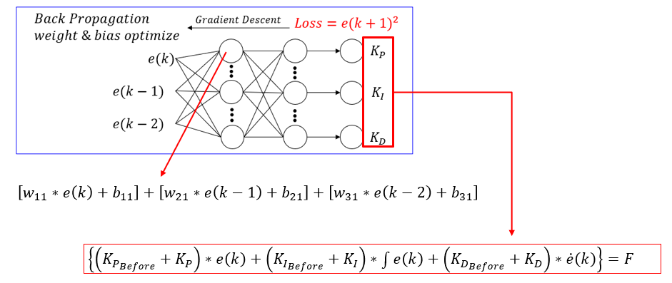
X1 defined at the beginning of the function is the input to the NN-Model.

\(\text{X}1=[\theta (k),\,\,\theta (k-1),\,\,\theta (k-2)]=[e(k),\,\,e(k-1),\,\,e(k-2)]\) Here \(\theta (k)\) means the angle at the pendulum at the kth step, and the target is 0, it is the same as the error value at the corresponding step \(e(k)\).

The next defined w and b values are the weights and bias values of the neural network model. In the code, w1, w2, b1, b2 are used to mean a model using a total of two hidden layers, and w3 means a channel to the output.

The learning rate and epoach each means to the value multiplied by the gradient of the loss and the number of learning times. The learning rate is expressed as a value that is directly multiplied by the gradient for the loss of each weight and bias \({{w}_{i}}={{w}_{i}}+\eta d{{w}_{i}}\,\,\,\eta =learning\,rate\).

The loss in the neural network model is represented by \({{w}_{i}}={{w}_{i}}+\eta d{{w}_{i}}\,\,\,\eta =learning\,rate\) as the angle of the pendulum in the next step. Here, the angle in the next step is obtained by directly finding it using the equation of motion. \((M+m)\,\left[ \frac{I+m{{l}^{2}}-mgl\phi }{ml}-g\phi \right]\,-\,ml\ddot{\phi }=u=F\,,\,\,\phi =\theta (k+1),\,\,\ddot{\phi }=\frac{\theta (k+1)-2\theta (k)+\theta (k-1)}{2}\)

The loss is calculated with the corresponding formula, and the training is repeated as many times as the number of epoachs updating while and bias with the gradient for the loss in the for statement.

# read the model description
model_description = read_model_description(fmu_filename)

# Initialize analysis parameter
var_input = {}
var_output = {}
start_time = 0.0
stop_time = 0.0
step_size = 0.0
ninput = 0
noutput = 0
ESum = 0

Read the fmu file in the specified path and define the necessary parameters.

for variable in model_description.modelVariables:
    if "RD_StopTimeDefined" in variable.name:
        stop_time = float(variable.start)
        stop_time = stop_time
    if "InterfaceStepSize" in variable.name:
        step_size = float(variable.start)
    if "nPinput" in variable.name:
        ninput = int(variable.start)
    if "nPoutput" in variable.name:
        noutput = int(variable.start)
    if "Input Data1 of Plant(RD)" in variable.description:
        var_input[variable.name] = variable.valueReference
    if "Output Data1 of Plant(RD)" in variable.description:
        var_output[variable.name] = variable.valueReference

Read the fmu file and set the model variable.

# IO variable reference to list
var_in = list(var_input.values())
var_out = list(var_output.values())

# extract the FMU
unzipdir = extract(fmu_filename)
fmu = FMU2Slave(guid=model_description.guid, unzipDirectory=unzipdir,
modelIdentifier=model_description.coSimulation.modelIdentifier, instanceName='instance1')

Unzip the fmu file.

# initialize
fmu.instantiate()
fmu.setupExperiment(startTime=start_time, stopTime = stop_time)
fmu.enterInitializationMode()
fmu.exitInitializationMode()

# simulation standby
time = start_time states = [[0 for \_ in range(len(var_in) + len(var_out) + 1)]]**

# states = np.zeros(len(var_in) + len(var_out))
outputs = [0 for \_ in range(len(var_out))]

Input_Theta = []
k = 0 Gain_P = -1000.
Gain_I = 0.
Gain_D = -125.

Initialize fmu for analysis and define the initial gain values of P,I and D and define the Input theta list to be used in NN-model.

# simulation loop
while time <= (stop_time + 1):
      inputs = np.zeros(len(var_in)).tolist()
      inputs, outputs = PIDControl(time, var_in, var_out, inputs, outputs, step_size, ESum, Gain_P, Gain_D, Gain_I)
      ESum += outputs[0] \* step_size Input_Theta.append(outputs[0])
      output_PID = np.array([Gain_P, Gain_I, Gain_D])
      output_PID = output_PID.reshape((1, 3))
      if k >= 3 :
         Gain_P_1, Gain_I_1, Gain_D_1 = NNModel(Input_Theta, output_PID, k,ESum,time,outputs,step_size)
         Gain_P = Gain_P - Gain_P_1
         Gain_I = Gain_I - Gain_I_1
         Gain_D = Gain_D - Gain_D_1
      time += step_size
      k += 1

# Simulation Terminate
fmu.terminate()
fmu.freeInstance()

Run Analysis.

5.1.5.4.3. Running Python File with Window Batch Command

In this part, we see how the results change as the learning rate and epoach change. In the previous FMPY_NN_Control.py file, set the learning rate to 0.01, change the epoach to 100 and save the file.

1. Run Windows Batch Command (CMD.exe).

2. Enter the following command to move to the folder where the *.py file is located.

   [Command: cd /d “<Path located py file>”]

3. Run the python file with the following command.

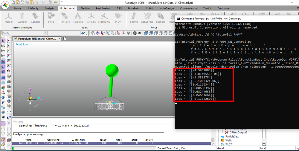
   [Command: py FMPY_NN_Control.py]

4. You can see the analysis in progress.

5. In the same way, change the learning rate to 0.01 and the epoach to 2000 and proceed with the analysis. Please note that it takes about 30 to 40 minutes.

6. If you proceed with the analysis, can check the change in the loss with the command line, and you can see that the loss decreases as the learning progresses.

   

5.1.5.4.4. Check the Result

1. Run RecurDyn.

2. Create a new model and click the Plot Result function in the Plot group of the Analysis tab.

3. Bring the two files that have been analysis (Learning rate=0.01 & epoach=100, Learning rate=0.01 & epoach=2000) together with the analysis result using \({{K}_{P}}=-1000,{{K}_{I}}=0,{{K}_{D}}=-125\,(PD\,Control)\) in the previous chapter.

4. Draw the GPlantOutput1 Value for each case in the Plot Database Window.

   

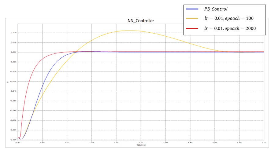
5. You can see that the more times you learn, the more accurate the learning and get the better results.

5.1.5.4.5. Running the Python File with Pycharm

When using the previous Windows Batch Command, the learning rate was fixed and the epoach was changed. Conversely, when proceeding with PyCharm, check the result when the epoach is fixed and the learning rate is changed.

1. Run Pycharm.

2. Open FMPY_NN_Control.py file in project. In the file FMPY_NN_Control.py, set the learning rate to 0.001 and the epoach to 2000.

   

3. Click the Run button or use the right-click on the project name to run the python file.

4. You can see the analysis in progress.

   

5.1.5.4.6. Check the Result

1. Run RecurDyn.

2. Create a new model and click the Plot Result function in the Plot group of the Analysis tab.

3. Bring the two files that have been analysis (Learning rate=0.01 & epoach=2000, Learning rate=0.001 & epoach=2000) together with the analysis result using \({{K}_{P}}=-1000,{{K}_{I}}=0,{{K}_{D}}=-125\,(PD\,Control)\) in the previous chapter.

4. Draw the GPlantOutput1 Value for each case in the Plot Database Window.

   

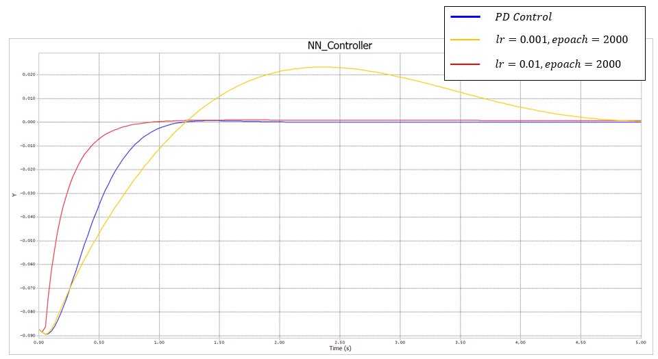
5. If you check the result, you can see that the loss is not reflected well if you use a low learning rate, so the result does not improve.