9.1. Riding Lawnmower with V-Belt Tutorial (Belt)

9.1.1. Getting Started

9.1.1.1. Objective

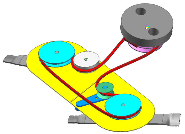
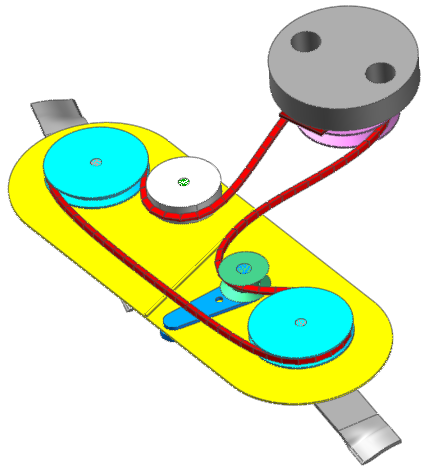
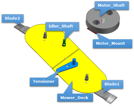
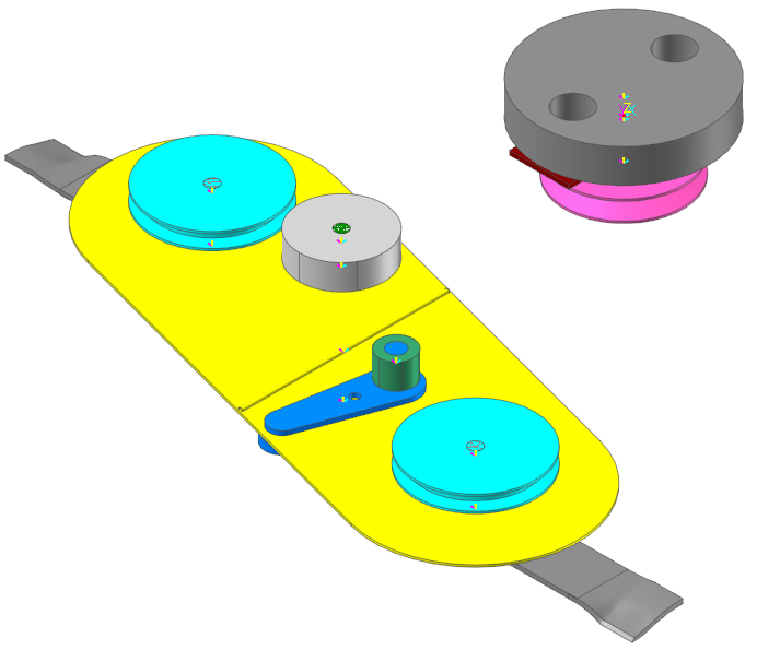
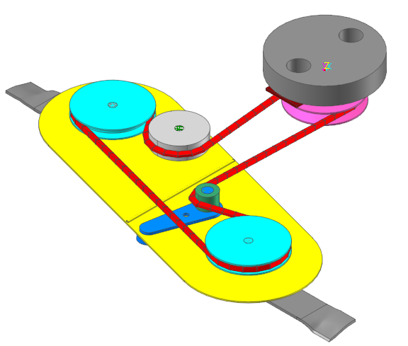
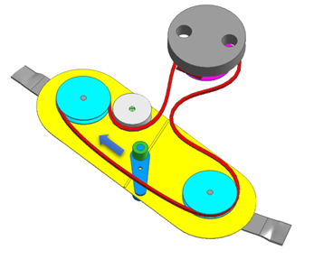
This tutorial will help you learn how to simulate the V-belt mowing system of a riding lawnmower using the RecurDyn Belt toolkit. You will generate animations and plots, which will provide insight into the function of the model and verify your intuitive understanding of the belt system. The completed V-belt mowing system is shown below.

The RecurDyn/Belt toolkit lets you model belt and pulley systems of various types and configurations. Some of the geometric entities in the toolkit that you will use in this tutorial include.

• V-belt

• Roller

• Flange

• V-pulley

RecurDyn automatically creates the contacts between these entities and the belt segments when you assemble the belt system. You can also use other RecurDyn bodies, constraints, and force elements to model the belt systems.

9.1.1.2. Audience

This tutorial is intended for experienced users of RecurDyn who previously learned how to create geometry, joints, and force entities. All new tasks are explained carefully.

9.1.1.3. Prerequisites

You should first work through the 3D Crank-Slider and Engine with Propeller tutorials, or the equivalent. We assume that you have a basic knowledge of physics.

9.1.1.4. Procedures

The tutorial is comprised of the following procedures. The estimated time to complete each procedure is shown in the table. We’ve also provided optional tasks to further refine the model. These optional tasks take approximately 25 minutes to complete.

Procedures	Time (minutes)
Creating the subsystem	5
Creating geometric entities	15
Assembling and simulating the V-belt	25
Refining the model	15
Total	60

9.1.1.5. Estimated Time to Complete

This tutorial takes approximately 60 minutes to complete, plus 25 minutes for the optional tasks.

9.1.2. Creating the Subsystem

9.1.2.1. Task Objective

Learn how to set up the simulation environment, create a subsystem of a belt, and import the geometry for the base plates (mower deck and motor mount) of the belt system.

9.1.2.2. Estimated Time to Complete

5 minutes

9.1.2.3. Starting RecurDyn

9.1.2.3.1. To start RecurDyn and create a new model:

1. On your Desktop, double-click the RecurDyn icon. RecurDyn starts and the Start RecurDyn dialog box appears.

2. Set the following.

   • Units: MMKS

   • Gravity: -Z

3. Save the file as Riding_Mower.

9.1.2.4. Creating a Belt Subsystem

You will now create a belt subsystem to contain the V-belt of the riding mower. You will import its geometry from a Parasolid file.

9.1.2.4.1. To create a belt subsystem:

1. From the Subsystem Toolkit in the Toolkit tab, click the Belt function. The modeling and Database windows only show the belt subsystem.

2. From the File menu, choose the Import function.

3. Set Files of type to ParaSolid File (x_t).

4. Select the file RidingMower.x_t.

   (The file path: <InstalDir>\Help\Tutorial\Toolkit\Belt\RidingLawnmowerWithVBelt)
   

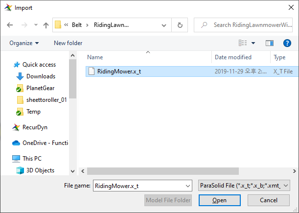
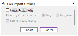
5. Click Open. The CAD Import Options window appears. Clear the Assembly Hierarchy checkbox and click Import.

   

6. Change the rendering mode to shade with wire.

7. Change the icon and marker size to 10. Your model should look like the following.

   

9.1.3. Creating the Geometric Entities

9.1.3.1. Task Objective

In this chapter, you will create the geometric entities that guide the V-belt.

• V-pulley

• Roller

• Flange

In the next chapter, you will assemble the V-belt elements and run a simulation.

9.1.3.2. Estimated Time to Complete

15 minutes

9.1.3.3. Creating the V-pulley

In this section, you create the V-pulley that attaches to the motor.

9.1.3.3.1. To create the V-pulley:

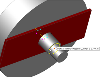
1. Starting from the default XY plane, rotate the model so that you can see the underneath of the Motor_Shaft body as shown in the figure below.

2. From the Pulley group in the Belt tab, click the V Pulley function.

3. Place your cursor on the center of the shoulder of the motor shaft.

   RecurDyn automatically selects the center of the circle that your cursor is on and, therefore, selects the center of the shaft as shown below.

   

   The V-pulley dialog box appears for specifying key dimensions of the V-pulley.

4. Click Dimension Information to view a description of what the dimensions represent.

   

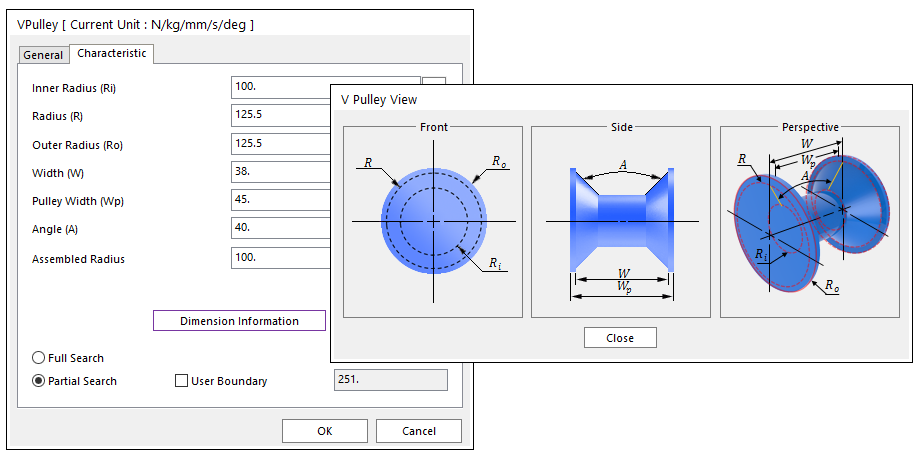
5. Click Close.

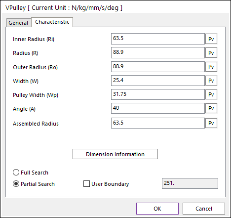
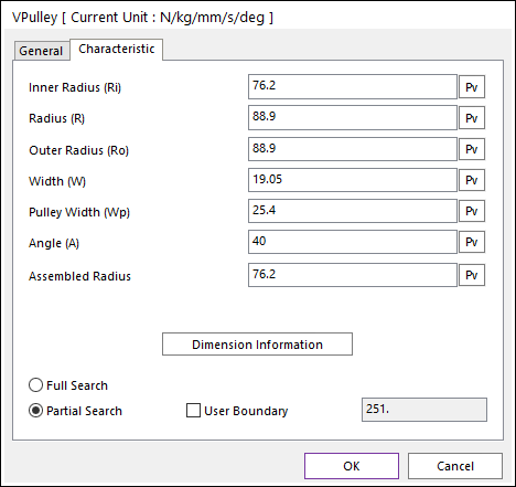
6. Enter the values as shown in the VPulley dialog box on the right and click OK.

   • Inner Radius: 63.5

   • Radius: 88.9

   • Outer Radius: 88.9

   • Width: 25.4

   • Pulley Width: 31.75

   • Angle: 40

   • Assembled Radius: 63.5

     

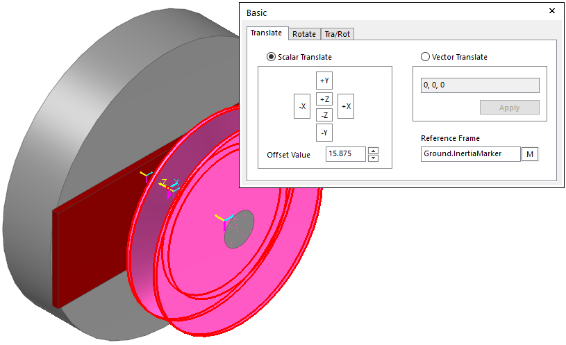
   By selecting the center of the shoulder as the creation point for the pulley, you have centered the pulley on this feature. You now need to offset the pulley so the edge of it is resting on the shoulder.

7. Using the Basic Object Control, move the pulley half the width (15.875 mm) in the negative z-direction. You will see that the bottom side of the pulley is aligned with the end of the motor shaft as shown in the figure below.

   

8. Similarly, create V-pulleys on the shafts of the two blades. Both have identical dimensions as those shown in the dialog box on the right. (Create VPulley2 on the top shaft, VPulley3 on the bottom Relative to XY plane.)

   • Inner Radius: 76.2

   • Radius: 88.9

   • Outer Radius: 88.9

   • Width: 19.05

   • Pulley Width: 25.4

   • Angle: 40

   • Assembled Radius: 76.2

     

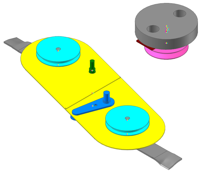
9. Make sure to offset both pulleys 12.7 mm in the positive z-direction to position them correctly on the shafts. Your model should now look like the following.

   

9.1.3.4. Creating the Roller

Create the roller on the tensioning link (shown in blue in the figure below).

9.1.3.4.1. To create the roller:

1. From the Pulley in the Belt tab, click the Roller function.

2. To fully define the roller during the creation process, change the creation method to Point, Distance, Depth.

3. Place the cursor on the shoulder of the shaft as you did before and select the center of the shaft as the center of the roller. Then, in the Input window toolbar at the top of the screen, enter 25.4 as the distance (radius) and 38.1 as the depth (height of the cylinder).

4. Offset the roller half the height (19.05 mm) in the positive z-direction.

   

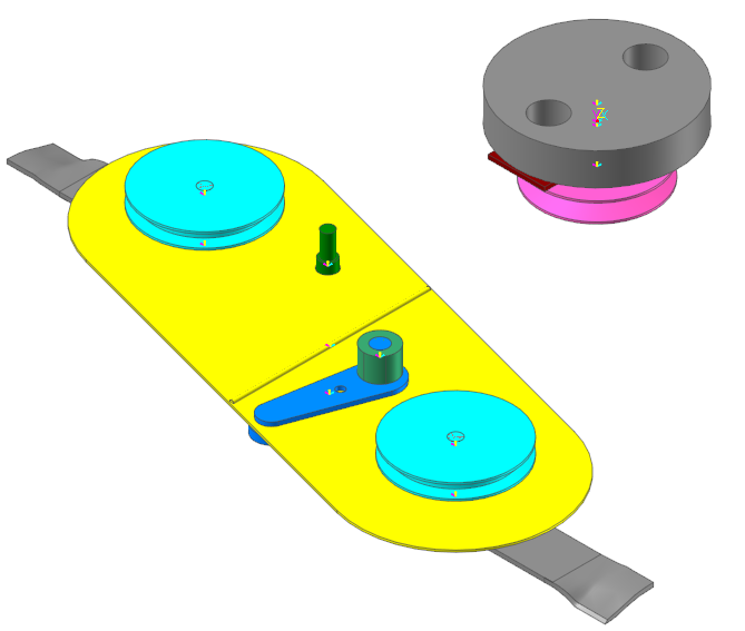
5. Similarly, create the roller on the dark green shaft (idler). Use the same creation method but this time, use 63.5 as the distance (radius) and 38.1 as the depth (height).

6. Offset the roller half the height (19.05 mm) in the positive z-direction.

9.1.3.5. Creating the V-belt Segment Definition

9.1.3.5.1. To create the V-belt segment definition:

1. From the Belt group in the Belt tab, click the V Belt function.

2. With the Working Plane set to the xy plane, select any point you want, preferably one slightly away from all of the components in the model.

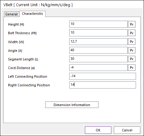
3. In the Properties dialog box that appears, enter the values as shown below to define the profile of the V-belt. These values yield a moderately coarse model of the belt. To further define it, shorten the segment length and adjust the connecting positions appropriately. The tradeoff is that a larger number of segments require a longer simulation time while providing smoother, more accurate results.

   • Height: 10

   • Belt Thickness: 10

   • Width: 12.7

   • Angle:40

   • Segment Length: 30

   • Cord Distance: -4

   • Left Connecting Position: -14

   • Right Connecting Position: 14

     

9.1.4. Assembling the Belt

9.1.4.1. Task Objective

In this chapter, you will create the belt and assemble the geometric entities that you created in the previous chapter. You will then run a simulation of the subsystem.

9.1.4.2. Estimated Time to Complete

25 minutes

9.1.4.3. Defining the Path for the Belt

9.1.4.3.1. To define the path of the belt:

1. Change the view to the xy plane and switch to the wireframe render mode.

2. Click the Assembly function of the Assembly group in the Belt tab.

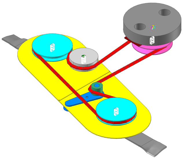
3. Click each individual roller along the belt’s path of travel, starting with the motor pulley and proceeding counterclockwise. Make sure that the thin blue line snaps to the correct side of the pulleys and rollers as shown in the figure on the below.

   

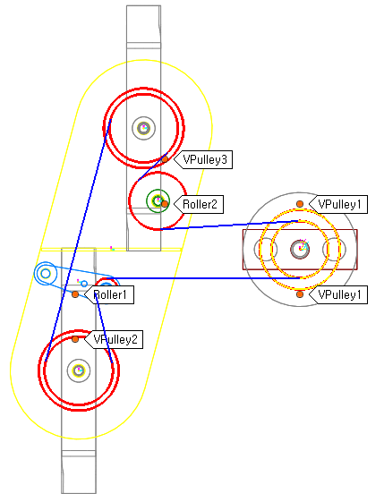
4. After you have selected all of the rollers, select the beginning pulley again, but this time with the blue line coming to the other side of the pulley hub to finish the loop. The dialog box shown on the below appears.

5. You want the belt to be slightly slack when the simulation begins, so change the number of belts (belt segments) to 94 instead of 93.

   

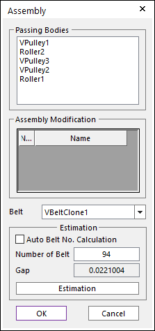
6. Click OK.

   RecurDyn adds bodies to the subsystem model for each individual belt segment. Your model should now look like the one shown next.

   

9.1.4.4. Fixing the Pulleys to Shafts

Now you fix the pulleys to their shafts.

9.1.4.4.1. To create fixed joints:

1. Click the Fixed Joint function of the Joint group in the Professional tab and create fixed joints as shown in the table below. Use the Body, Body, Point method.

   	Body 1 (base)	Body 2 (action)	Point
   FixedJoint1	Motor_Shaft	VPulley1	0, 0, -60.325
   FixedJoint2	Blade2	VPulley2	VPulley2.CM
   FixedJoint3	Blade1	VPulley3	VPulley3.CM
   FixedJoint4	Idler_Shaft	Roller2	Roller2.CM

2. Do this for each of the three pulleys but only for the gray (bigger) roller. The green (smaller) roller needs to spin freely on the blue arm, which then pivots around its mounting location on the mower deck to engage and disengage the belt from the motor.

   

9.1.4.5. Creating Revolute Joints

Now you will create revolute (pin) joints between each of the shafts and the base plate to which they are mounted. You will also create a pin joint between the green roller and the blue arm as discussed in the previous step.

9.1.4.5.1. To create revolute joints:

• Click the Revolute Joint function of the Joint group in the Professional tab and create revolute joints as shown in the table below. Use the Body, Body, Point method. Selecting a center of circle on each shaft gives you pin joints that rotate about the centerline of each shaft.

  	Body 1 (base)	Body 2 (action)
  RevJoint1	MotherBody	Motor_Shaft
  RevJoint2	Mower_Deck	Blade2
  RevJoint3	Mower_Deck	Blade1
  RevJoint4	Mower_Deck	Tensioner
  RevJoint5	Tensioner	Roller1
  RevJoint6	Mower_Deck	Idler_Shaft

  

9.1.4.6. Connecting the Motor Mount and Mower Deck to Ground

The Motor_Mount plate will be fixed directly to the MotherBody, which will be considered ground.

The yellow Mower_Deck, on the other hand, needs to have some freedom of motion so that it can adapt to varying terrain. You will simulate this effect by creating a revolute joint along the center axis of the plate. A semicircular ridge is on this axis to simplify the joint creation process.

9.1.4.6.1. To connect the base plates to ground:

1. Create a Fixed joint anywhere on the Motor_Mount plate.

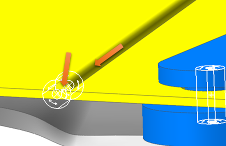
2. Create a revolute joint using the Point, Direction creation method for the Mower_Deck. First, select the semicircular center of the ridge and then select the ridge itself to specify the direction.

   You will start the simulations with the simplest case by specifying the motion of this joint as zero. This makes it essentially a fixed joint, but one that you can easily modify later.

   

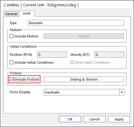
3. Right-click the revolute joint and select Properties.

4. Select Include Motion and then specify the function expression as zero to indicate that there will be no motion for this simulation. If you have any questions about the process, please refer to the section below for a review of defining a joint motion with a function expression.

9.1.4.7. Applying Motion to the Motor Shaft

Now you will set the motor speed to ramp up to 1800 rpm by modifying the motion of RevJoint1 between the Motor_Mount plate and the Motor_Shaft.

9.1.4.7.1. To get the motor running:

1. In the Database Window, right-click RevJoint1, and click Properties.

2. Click Include Motion, and then click Motion.

3. Set the motion type to Velocity (time).

4. Set the expression for the motion as shown in the figure on the below.

   • -188.4*STEP(TIME, 0, 0, 1, 1)

     

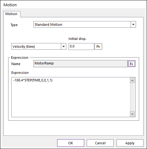
5. Click OK twice to exit.

   This ramps up the motor speed from zero to 188.4 rad/s in one second.

9.1.4.8. Applying a Force to the Tensioner Link

Now, you will create a force at the hole located roughly 2/3 of the way between the pivot and the roller. This force will engage the belt and drive the blades. The force represents a cable/lever/spring system that is not included in this model. The value of this force determines the tension in the belt and has a significant effect on the slipping between the belt and the motor shaft. This force value would make an excellent parameter to vary in a design study.

9.1.4.8.1. To create the force:

1. Click the Axial Force function of the Force group in the Professional tab and create the axial using the default creation method Body, Body, Point, Point.

2. Click tensioner and then click Mower_Deck.

3. For the first point, select the hole in the tensioner where the spring would attach. For the second point, select any point on the Mower_Deck because you will change its location in the next step.

4. Display the Properties dialog box of the newly created axial force, click the Connector page, and change the location (Origin) of the Action (second) marker to (-400, 200, -85.725) as shown in the figure on the below.

   

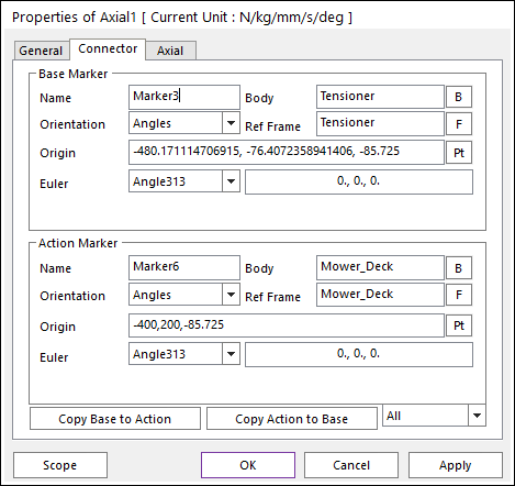
   This makes the force roughly tangent to the initial direction of motion for the tensioner, maximizing the mechanical advantage.

   Typically, when the mower is turned on, first the motor comes up to speed with the belt slipping so no torque is transmitted to the blades. Then, the blades are engaged by applying the proper force to the tensioner link.

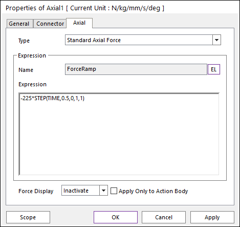
   You will simulate this by ramping up the force from zero to 225 N (~50 lb) when the motor is almost up to speed (0.5 seconds into the simulation).

5. In the Properties dialog box, click the Axial page.

6. Enter the function expression as shown in the figure on the below.

   • -225*STEP(TIME, 0.5, 0, 1, 1)

     

9.1.4.9. Running the Simulation

You are now ready to run the simulation for the first time.

9.1.4.9.1. To run the simulation:

1. From the Simulation Type group in the Analysis tab, click the Dynamic / Kinematic Analysis function.

2. Set the simulation to run for 1.25 seconds with 200 steps as shown in the figure on the below. This will give the motor sufficient time to come up to its full speed.

   

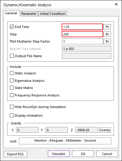
3. Click Simulate.

The simulation runs in a little less than 10 minutes on a 2.6 GHz Pentium 4 processor.

9.1.4.10. Viewing the Results

9.1.4.10.1. To view the results:

• Click the Play function of the Animation Control group in the Analysis tab at the top of the window to play the results.

  

Looking at the results of the simulation, notice that there is a significant design flaw with this mower. The belt is unable to stay in place on the tensioner roller because there are no flanges to hold it there. In the next chapter, you will modify this roller so it has appropriate flanges.

9.1.5. Refining the Model

9.1.5.1. Task Objective

In this chapter, you will refine the model by adding flanges to the tensioner roller and rerun the simulation. You will then plot the results.

9.1.5.2. Estimated Time to Complete

15 minutes

9.1.5.3. Adding Flanges to the Rollers

To make room on the roller for the flanges, you will first need to decrease its width (height). Then, you will create the flanges, adjust their sizes, and fix them to the roller.

9.1.5.3.1. To add flanges to the roller:

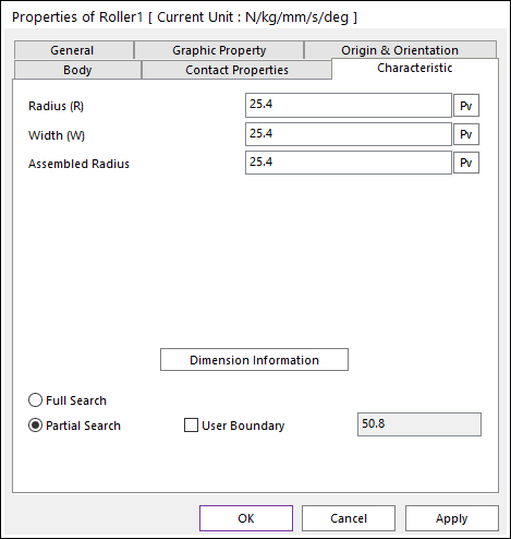
1. Right-click the small green roller and click Properties. In the Properties dialog box, click the Characteristic page, and change its width to 25.4 as shown in the figure on the below.

   

   Now, add the flange.

2. From the Pulley group in the Belt tab, click the Flange function.

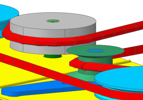
3. Click the top face of the roller. Repeat for the bottom face of the roller.

   The default size for the flanges is far too large for this application.

4. Right-click the flanges, select Properties, and in the Characteristics page, change the depth (Width) of the flanges to 6.35 mm.

   

5. Connect each of the flanges to the roller body with a fixed joint.

9.1.5.4. Modifying the Belt

For the flanges or the flanges to work properly, you need to modify the belt assembly so that it knows to include possible contact with the two flanges.

9.1.5.4.1. To modify the belt assembly:

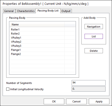
1. Scroll down to the bottom of the Database Window, right-click BeltAssembly1, and then click Properties.

   Because you have added flanges to the rollers, you need to tell RecurDyn to look for contact with these additional bodies.

2. Add the bodies shown in the figure on the below using either the Navigation or List options and click OK.

   

9.1.5.5. Adding Friction to the Blade Joints

You may have noticed that in the previous simulation that the blades moved freely from the moment the motor started turning. This is not realistic. On an actual mower, there would be a brake to hold the blades in place until the force is applied. Modeling this geometry is beyond the scope of this tutorial.

Friction is also left out of this model, however, and you will add it to provide resistance to the blade motion so you can see the effect of applying the force to the tensioner.

9.1.5.5.1. To add friction:

1. Display the Properties dialog boxes for the revolute joints between the Blades and the Mower_Deck (should be RevJoint2 and RevJoint3).

   By default, the effective moment arms for the friction are too high.

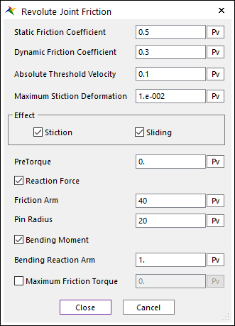
2. Check Include Friction.

   

3. Click the Sliding & Stiction button to change the values to match the figure on the below.

   You will leave the other values at their default.

   • Friction Arm: 40

   • Pin Radius: 20

     

4. Click Close and then select OK. You are now ready to run the simulation again.

5. Run the simulation again with the same settings as before (1.25 second with 200 steps).

   When you play the animation, you will see that the belt is operating properly. The flanges are keeping the belt from moving off of the roller on the tensioner.

9.1.5.6. Viewing the Results

You will now view the results.

9.1.5.6.1. To view the results:

1. Click the Plot Result function in the Analysis tab to open the Plot Window so you can add display data curves of the motor speed and blade speed.

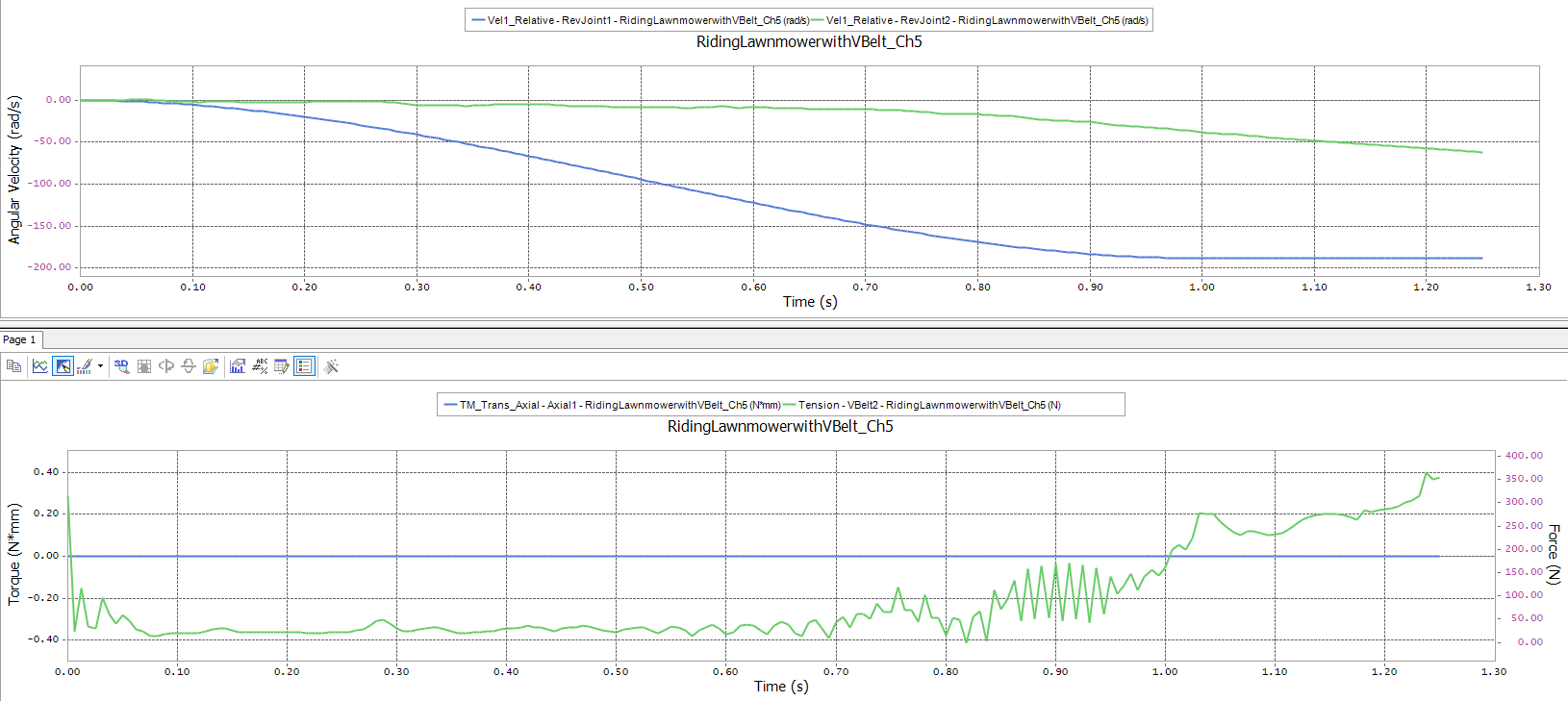
2. Draw the Vel1_Relative values of RevJoint1 (motor speed) and RevJoint2 (blade speed).

3. Click the Show left Windows function in the Windows group of the Home tab to divide the window into two panes.

   Add the applied axial force and belt tension to the second (lower) pane.

4. Click the lower pane to activate it.

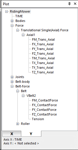
5. Draw the FM_Trans_Axial of the Axial1 force and draw the Tension of the VBelt2 belt segment (see the figure on the below for assistance).

   

   You should be able to see that when the force is applied to the tensioner, the belt tension increases, and the mower blades start coming up to speed. It looks like the blades did not quite come up to speed yet, but they are clearly performing as desired. To see what the steady-state speed of the blades is, run the simulation for a longer time. Alternatively, you could increase the tensioner force value, friction coefficients, or moment arms so the belt stops slipping sooner.

6. From the System menu, choose Close to return to the modeling environment.

You now have a working model of a riding lawnmower blade drive train. The following chapter contains optional tasks.

9.1.6. Performing Optional Tasks

9.1.6.1. Task Objective

In this chapter, you will further refine the model by adding oscillatory motion to the MowerDeck. You will also create a slip sensor, request output data for additional belt segments, and make plots of the results.

9.1.6.2. Estimated Time to Complete

25 minutes

9.1.6.3. Creating a Slip Sensor

You will create a sensor to measure the slip between the belt and the motor V-pulley.

9.1.6.3.1. To create the sensor:

1. From the Sensor group in the Belt tab, click the Slip Sensor function.

2. Set the Creation Method to RollerBody, Point, Distance.

3. Enter three inputs:

   • RollerBody - Select the motor VPulley1.

   • Point (Sensor location) - Choose a point on the same level (z-direction) as the pulley center and on the other side of the belt from the pulley (160, 0, -60.325).

   • Distance (Search radius) - Select 100.

     The sensor icon is now present, but before it is functional, you need to specify which belt it is to sense.

4. Right-click the sensor icon and select Properties.

5. In the Properties dialog box, next to Sensed Entity text box, click E, and then click any segment of the belt.

   BeltAssembly1 appears in the Sensed Entity text box as shown in the figure on the below.

   

6. Click OK.

   You are ready to simulate.

   Running the simulation for 2.5 seconds allows the system to come closer to equilibrium, so if you have enough time to wait as the simulation runs, go ahead and use that as the simulation time. If you are going to do the next section, it is recommended that you wait to run the simulation because a simulation is included at the conclusion of that section as well.

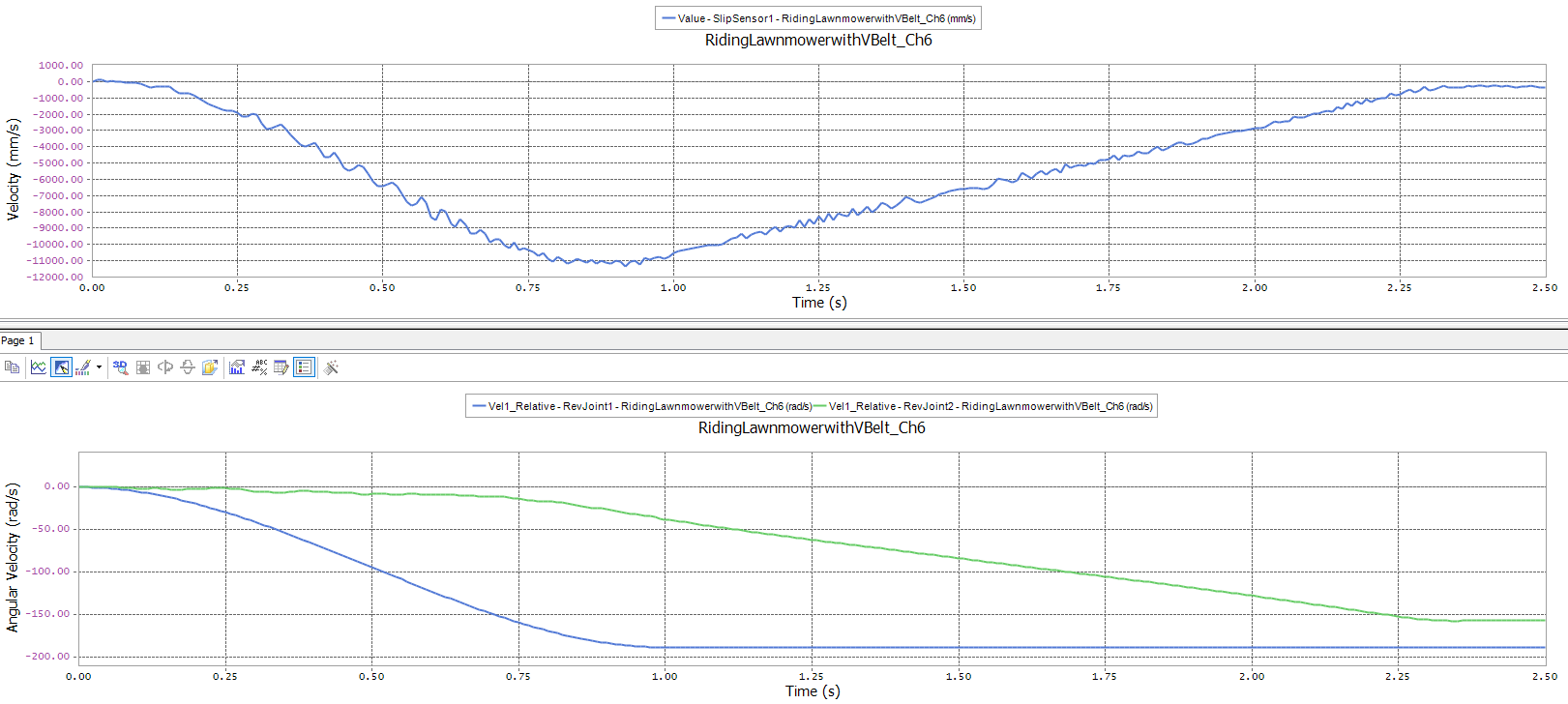
7. (Optional) Run the simulation for 2.5 seconds with 300 steps. The following plots show the results of this simulation.

8. Draw the Value of the SlipSensor1 in the upper window and draw the Vel_Relative of RevJoint1 and RevJoint2 in the lower window.

   The upper plots show that the maximum slip for the drive pulley occurs at approximately 0.85 seconds. The lower plot shows that the blade velocity gets closer to the belt velocity with the longer simulation time.

   

9.1.6.4. Requesting Output Data for Additional Segments

Track the tension in multiple belt segments by requesting the data from RecurDyn.

9.1.6.4.1. To track the tension:

1. In the Database Window, right-click BeltAssembly1, and select Properties.

   
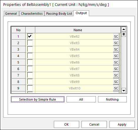
2. Click the Output page and check the boxes next to the belt segments for which you would like the output data. To keep it simple, select only three segments: VBelt2, VBelt32, and VBelt62.

   Now that RecurDyn knows to store the output data for these segments, run the simulation.
3. Run the simulation (2.5 seconds with 300 steps).

   Because you now have data for these three links, you need to visually mark them so you can identify them in the animation. You do this using Render Each mode.

4. Click the Each Render tool in Render Toolbar.

5. Set the entire belt assembly to wireframe by clicking the first link (VBelt2) in the Database window, scrolling down, and then, while holding down the Shift key, clicking the last link (VBelt95).

6. Now that you have selected all 94 links, right-click one of them and click Properties for the segments.

7. Click the Graphic Property page and set Each Rendering to Wireframe as shown in the figure on the below.

   

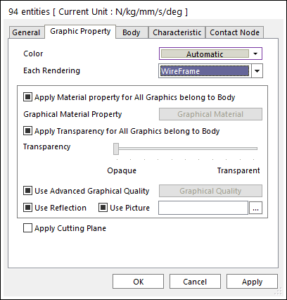
8. Click OK to exit the Properties dialog.

9. Define Set the desired links (VBelt2, VBelt32, and VBelt62) to be shaded by right-clicking each of their entries (one at a time) in the Database window and selecting clicking Shade from the pop-up menu.

10. Set the shading rendering mode for all the other bodies to shaded, except the Mower_Deck. Setting the Mower_Deck to wireframe allows you to better visualization of the lawnmower blades.

9.1.6.5. Viewing the Results

In this section, you will plot the belt tension for the three selected segments, the pulley velocities, the tensioner force, and include the animation. The most effective way to view these elements is to plot the segment tensions in one window of a split frame plot and have the animation in another. You can then quite easily see where the segments are as the tension in them changes. For example, as a segment passes over the motor V-pulley, it transitions from having a high tension to having a low tension so there is a positive net torque from the motor to the belt.

9.1.6.5.1. To view the results:

1. Open the Plot Window.

2. From the Windows group in the Home tab, click the Show All Windows function to divide the window into four panes.

3. Click in the top left pane to activate it.

4. Load the animation by clicking the Load Animation function of the Animation group in the Tool tab.

   A warning will be generated appears about deleting the view in that pane.

5. Since because there is nothing in the plot, and this is not a concern; click Yes to proceed. Modify the view and rendering mode of the animation using the same commands and tools you would normally use in the modeling environment.

6. Modify the view and rendering mode of the animation using the same commands and tools you would normally use in the modeling environment.

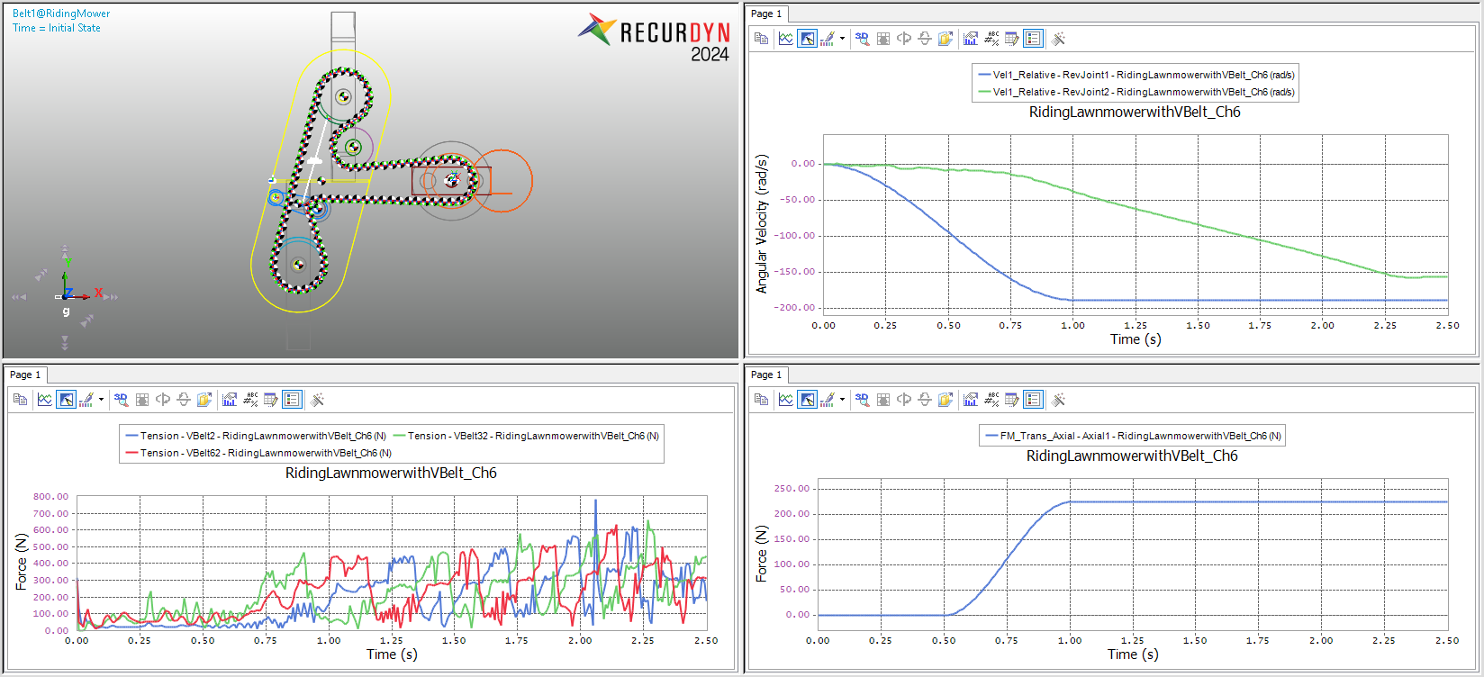
7. Click the bottom left pane to activate it and draw the Tension for the three belt segments (see the figure on below).

   

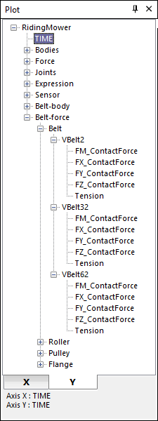
8. Click the top right pane to activate it and draw Vel1_Relative for RevJoint1 and RevJoint2 (motor and Blade2, respectively).

9. Click the bottom right pane to activate it and draw the tensioner force (FM_Trans_Axial for Axial1).

10. The following next figure shows the resulting plot.

    

9.1.6.6. Oscillating the Mower Deck

9.1.6.6.1. To oscillate Mower_Deck:

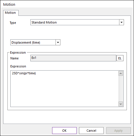
1. Modify the motion of the revolute joint connecting Mower_Deck to ground. Specify the motion as being sinusoidal with a period of two seconds and amplitude of 25 degrees.

   • (25D*sin(PI*TIME))

     

2. Return the simulation for two seconds to see the effects of the oscillation. Check how the tension in the belt and the position of the belt tensioner changes as the Mower_Deck oscillates.