7.3. Bimetal Thermometer (FFlex)

7.3.1. Overview

7.3.1.1. Objective

In multi-body dynamics analysis using a flexible body, if thermal deformation is considered, complex simulations on more diverse subjects are possible. The RecurDyn/FFlex Heat Transfer Toolkit includes several heat transfer methods that can be applied to flexible bodies. Let’s try TMFBD (Thermal Muti-Flelxible Body Dynamic) analysis, which integrates heat, flexible body, and multibody dynamics.

In this tutorial, you will learn how to perform structural analysis with a flexible body to account for heat transfer. First, load an existing model composed of a rigid body, and use Mesher to make a body to be deformed by heat among the rigid bodies into an FFlex body. You will see how this FFlex Body affects the overall structure.

In this tutorial, you will learn how to:

• Create a flexible body using manual meshes

• Set properties for thermal analysis

• Add Joint and Thermal Condition

• Create Expression Scope to check result

• View the results of the simulation

7.3.1.2. Prerequisites

This tutorial is intended for users who are familiar with the Professional and FFlex tutorials provided by RecurDyn. Therefore, before using this tutorial, you must precede the aforementioned tutorials in order to increase your understanding of this tutorial. It also requires an understanding of dynamics, finite element method, and heat transfer.

7.3.1.3. Procedures

The tutorial is comprised of the following procedures. The estimated time to complete each procedure is shown in the table.

Procedures	Time (minutes)
Generating an FFlex body	25
Creating Boundary and Thermal condition	10
Simulating the Model	10
Total	45

7.3.1.4. Estimated Time to Complete

This tutorial takes approximately 35 minutes to complete.

7.3.2. Generating an FFlex body

7.3.2.1. Objective

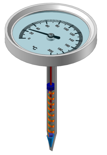
Open the initial model to check the configuration of a basic bimetal thermometer and try to make the bimetal body into a flexible body.

7.3.2.2. Estimated Time to Complete

25 minutes

7.3.2.3. Opening the RecurDyn Model

7.3.2.3.1. To run RecurDyn and open the initial model:

1. On the Desktop, double-click the RecurDyn icon. RecurDyn starts up and the Start RecurDyn dialog box appears.

2. Close the Start RecurDyn dialog box.

3. In the File menu, click Open.

4. Navigate to the FFlex tutorial folder and select BimetalThermometer_Start.rdyn.

   (The file path: <InstallDir>\Help\Tutorial\Flexible\FFlex\BimetalThermometer)

5. Click Open to open the model shown in the following figure.

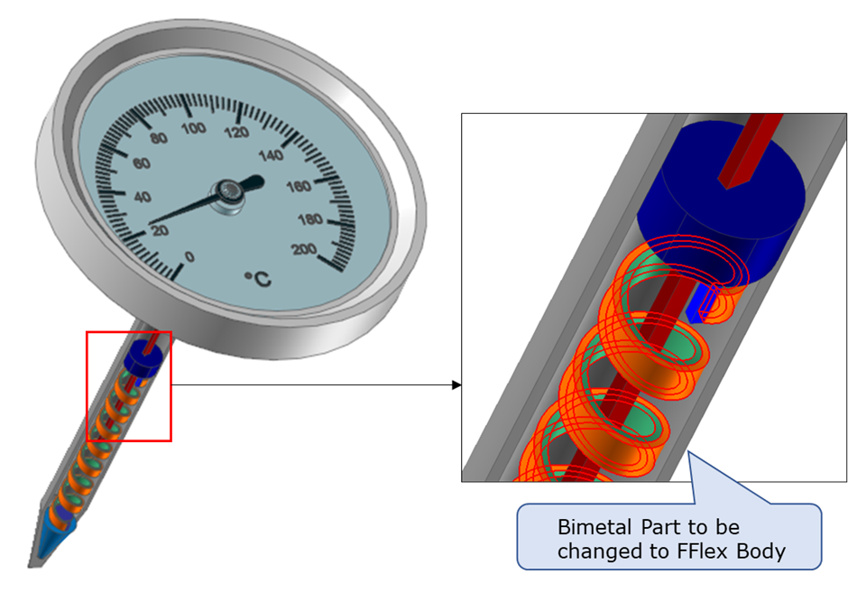
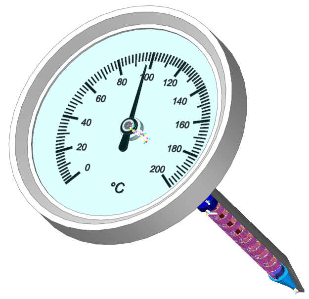
The bimetal of the thermometer shown below is a rigid body that will later be made into a FFlex body in this model.

7.3.2.3.2. To save the model:

1. In the File menu, Click Save As.

2. You cannot perform the simulation if the model is in the tutorial path, so you must save the model in a different path.

7.3.2.4. Creating the Bimetal Mesh

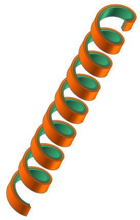
In this section, you make an FFlex body by referring to the rigid bimetal body to implement the deformation of bimetal. You will create a mesh using Advanced Mesh and Manual Mesh to create a uniform cubic element for a body that is not simple in shape.

7.3.2.4.1. To create Surface Mesh:

1. From the Mesh group in the Flexible tab, click the Mesher function.

2. Select the Bimetal body in Working window or, type Bimetal in Command Input window.

3. Click Yes in the pop-up window.

4. Mesh mode displays only the Bimetal Body, as shown below.

   

5. Click the Face Surface function from the Surface group in the Geometry tab.

6. Select Metal_1 to open FaceSurf Operation dialog window. With the FaceSurf Operation dialog window open, select Metal_1.Face6 at the bottom of the body.

   

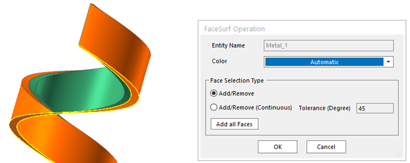
7. Click OK to create FaceSurface1.

8. Repeat the above process for Metal_2.Face6, which is the bottom of Metal_2, to create a FaceSurface2.

   

9. On the Mesher tab, click the Advanced Mesh function to open the Advanced Mesh dialog window.

   

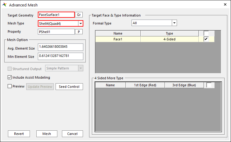
10. In the Mesh dialog window, perform the following:

    • In the Target Geometry option, Click Gr. Select FaceSurface1 in the Working Window.

    • In the Mesh Type dropdown menu, select Shell4(Quad4).

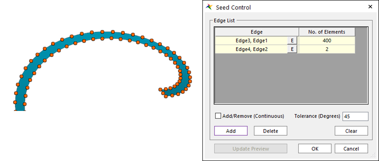
11. Click Seed Control. In the Seed Control dialog window, perform the following:

    • Click Add and select Edge (Edge1, Edge3) of Helix curve in the Working Window. After being added to the Edge List, set the No. of Elements to 400.

    • After adding the short edges (Edge2, Edge4) connecting the Helix curve to the list in the same way, set No. of Elements to 2.

    • Click OK.

    

12. Click Mesh in the Advance Mesh dialog.

13. Repeat the 10.-12. procedures for FaceSurface2.

14. Click Cancel to close Advanced Mesh dialog.

7.3.2.4.2. To create Manual Mesh:

1. Click the Extrude Manual Mesh function from the Mesher group. Extrude Manual Mesh dialog box appears.

2. Change the setting in Extrude Manual Mesh dialog as following:

   • Click Curve/Surface Type in Select Type.

   • To set FaceSurface1 to Entity, click E and select FaceSurface1 in the Working Window.

   • Enter PSolid1 in Property.

   • Enter 0,1,0 in Direction.

   • Enter 6 in No. of Segments.

   • Enter 3 in Total Length.

   • Uncheck Maintain Source Mesh option.

     

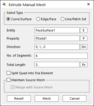
   • Click Mesh.

   • Click Cancel.

3. Click the Property function from the FFlex Edit group. Property dialog box appears.

4. Change in Property dialog as following:

   • Click Add. After the type dialog appears, select PSOLID type and click OK.

   • Double-click the Name column of the added property and input PSolid2.

   • Double-click the Material column of PSolid2, enter Mat_Property_3 and click OK.

     

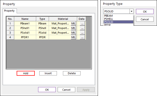
5. Repeat steps 1.-2. in the same way for the FaceSurface2 entity, but change the Property to PSolid2.

6. Click the Flex Merge function from the Mesher group. Flex Merge dialog box appears.

7. Change the setting in Flex Merge dialog as following:

   • Set Target Topology to Topol_1.

   • In Source Topology, check Sel. of Topol_2.

     

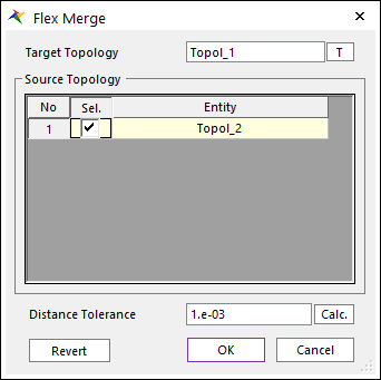
   • Click OK.

7.3.2.4.3. To create Node Set:

1. Click the Node Set function from the Set group.

2. Click Add/Remove (Continuous) in Node Set dialog.

3. As shown in the figure below, among the flat faces of the Bimetal, click the upper face in the Y direction.

   

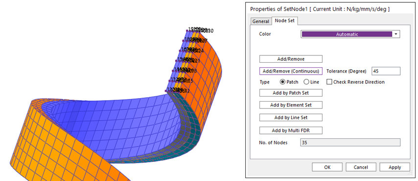
4. Click the right mouse button and select Finish Operation from the Pop-up Menu.

5. Click OK in Node Set dialog.

   • Confirm that SetNode1 has been created in Database.

6. Repeat steps 1.-5. in the same way for the lower face in the Y direction.

   • Confirm that SetNode2 has been created in Database.

7.3.2.5. To create FDR:

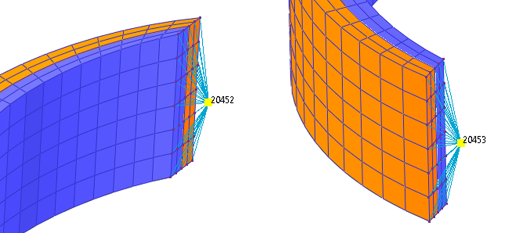
1. Click the Node function from the FFlex Edit group. Node dialog box appears.

2. Enter -0.5, -78.5, 3.5 for Position in the Node dialog.

   

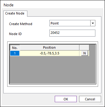
3. Click OK and confirm that the node has been created.

4. Click the FDR function from the FFlex Edit group.

5. Change the setting in FDR Creation Dialog as following:

   • After clicking N of Master Node, enter 20452 in the Input Window Toolbar.

   • After clicking N of Node Set, enter SetNode1 in the Input Window Toolbar.

     

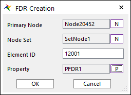
   • Click OK to close the dialog.

6. Repeat steps 1.-5., but with some changes to the following to create additional FDR.

   • Node Position: 0.5, -142.5, 3.5

   • Master Node: 20453

   • Node Set: SetNode2

   

7.3.2.6. Setting Material Property

You created an Element Property to create two other Solid Elements in Manual Mesh. In order to realize the physical change of Bimetal by temperature, you will change the Material Property.

1. Click the Material function form FFlex Edit group.

2. Change the setting in the Material dialog as following:

   • In No. 3, change the name of Mat_Property_3 to Mat_Metal_1.

   • Click Add, and change the name of Mat_Property_4 to Mat_Metal_2 in No. 4.

   • Click … in the Data column of Mat_Metal_1 to change the settings as follows.

     

     • Thermal Coefficient: 2.2e-005

     • Thermal Conductivity: 6000

   • Click Close to close Elastic - Isotropic dialog box.

   • Click … in the Data column of Mat_Metal_2 to change the settings as follows.

     

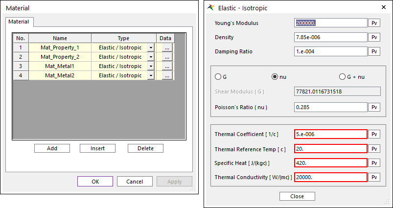
     • Thermal Coefficient: 5.e-006

     • Thermal Conductivity: 20000

   • Click Close to close Elastic - Isotropic dialog box.

   • Click OK to close Material dialog box.

3. Click the Property function form FFlex Edit group. Property dialog box appears.

   

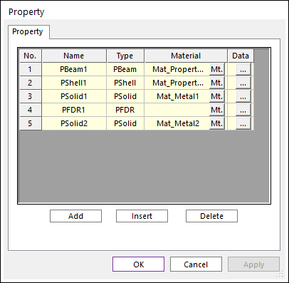
4. Change the settings in Property dialog box as following:

   • Enter Mat_Metal1 in Material of Psolid1.

   • Enter Mat_Metal2 in Material of Psolid2.

5. Click OK.

7.3.2.7. Creating the Patch Set

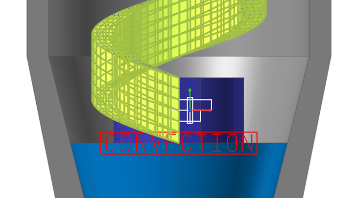
Before using the Thermal Feature of FFlex, you need to create the required Node Set or Patch Set according to the thermal type you want to create. In order to apply one Convection to Bimetal, you will create a single Patch Set for all faces except the faces that come into contact with Rigid Body.

1. Click the Patch Set function form Set group. Patch Set dialog box appears.

   

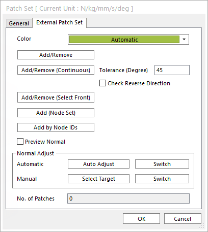
2. Click Add/Remove (Continuous) in Patch Set dialog box.

3. Select all faces except the face that created the Node Set.

4. Click the right mouse button and select Finish Operation from the Pop-up Menu.

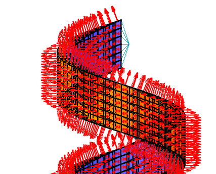
5. Click Preview Normal in Patch Set dialog.

6. Make sure all vertical lines are pointing out of the Surface, as shown in the figure on the below. Otherwise, click Auto Adjust to correct all vertical lines in the same direction as shown. If the direction is not what you want, click Switch to change the direction.

   

7. Click OK.

8. All work of Mesher has been completed. Click the Exit function.

7.3.3. Creating Boundary and Thermal Conditions

7.3.3.1. Task Objective

In this chapter, you will create joints for connecting the created Bimetal Mesh with the thermometer body and a Convection for thermal analysis.

7.3.3.2. Estimated Time to Complete

10 minutes

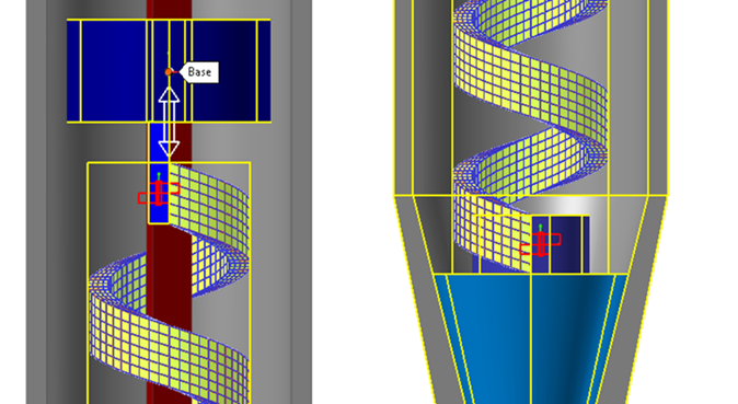
7.3.3.3. Creating the Fixed Joint

You will connect the Bimetal Mesh with the Rigid Body. Since both ends of the bimetal are fixed to different rigid bodies, you will make two fixed joints using the FDR you created earlier.

1. Click the Fixed Joint function from the Joint group in the Professional tab.

2. After setting Creation Method to Body, Body, Point, enter the following values in the Input Window Toolbar.

   • Slider

   • Bimetal

   • -0.5, -78.5, 3.5

3. When inputs are completed, Fixed1 is created as shown in the figure below.

4. Repeat steps 1.-2. to create Fixed2. Change the input value as follows.

   • Head_OutShaft

   • Bimetal

   • 0.5, -142.5, 3.5

5. When inputs are completed, Fixed2 is created.

7.3.3.4. Creating Convection

Bimetal is not in direct contact with the object to be measured in the current thermometer being modeled. However, for efficient simulation, you will not consider all heat transfer from the object to the thermometer shaft and to the bimetal. You will model the transfer of heat by convection between the surface of the Bimetal and the fluid, simplifying the overall process.

1. Click the Convection function from the FFlex group in the Flexible tab.

2. Change the setting in Convection dialog box as following:

   • In Patch Set, click P.

   • Enter Bimetal.SetPatch1 in the Input Window Toolbar.

   • Enter 1000 in Heat Coefficient.

   • Enter 100 in Ambient Fluid Temperature.

     

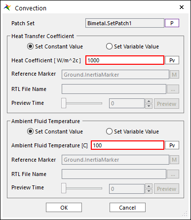
3. Click OK.

4. Confirm that Convection1 is created in Database Window.

   

7.3.4. Simulating the Model

7.3.4.1. Task Objectives

In this chapter, you will run a simulation of the created model. You will check the result by looking at the value indicated by the temperature guide with the scope.

7.3.4.2. Estimated Time to Complete

10 minutes

7.3.4.3. Creating the Expression Scope

You will create a Scope so that you can verify that the thermometer’s temperature reading is a good representation of the convective temperature. Because Expression Scope plots Expression values ​according to time, Expression must be defined before analysis. Learn how to create a scope after expressing the direction indicated by the temperature guide using Expression before performing the analysis.

The Pointer body of this model points to 20°C by default, and the gauge scale is drawn from 0°C to 200°C in 270°. The Pointer body is connected to the Head_OutShaft body by a revolute joint and rotates with a Z-direction (local). If the YAW angle, which is the Z-direction rotation, exceeds 180°, the value increases from -180°. Therefore, when the rotation angle of the temperature guide is 1 rad or more in the counterclockwise direction (in the section below 0°C) based on the default position of the pointer (20°C), the yaw angle is expressed as a continuous value in the clockwise direction. Considering the above, create an Expression representing the value pointed to by the guideline.

1. Click the Expression function from the Expression group in the SubEntity tab. Expression List dialog box appears.

2. Click Create in the dialog.

3. Enter the following values in Expression dialog box.

   • Name: Pointed_Temperature

   • Expression: 20-(yaw(Pointer.Marker1,Head_OutShaft.Marker3)

     +IF(yaw(Pointer.Marker1,Head_OutShaft.Marker3)-1:0,0,-2*PI))*RTOD*200/270
     

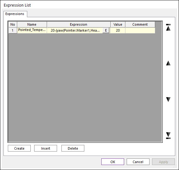
4. Click OK. In the dialog that appears next, click OK to finish writing the Expression.

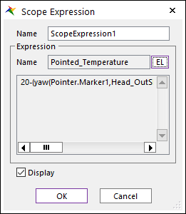
5. Click the Expression Scope function from the Scope group in the Analysis tab.

6. Click EL. Expression List dialog box appears.

7. Select Pointed_Temperature expression and click OK.

8. Confirm that the selected Expression is applied to the Scope Expression dialog box and click OK.

   

7.3.4.4. Performing Dynamic Analysis

You will run the simulation as follows to confirm that the generated model correctly displays the temperature guide according to the convection temperature.

7.3.4.4.1. To run the simulation:

1. Click the Dynamic / Kinematic Analysis function from the Simulation Type group in the Analysis tab.

2. Change the setting on the General page as following:

   • End Time: 10

   • Step: 100

   • Plot Multiplier Step Factor: 1

   • Output File Name: 100dC

     

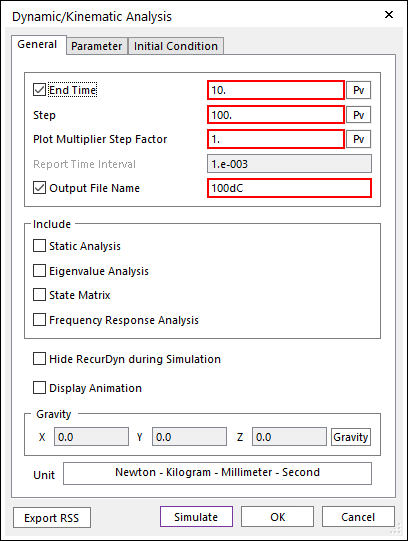
3. Click Simulate to run analysis.

7.3.4.4.2. To view the animation:

• Click the Play / Pause function from the Animation Control group in the Analysis tab.

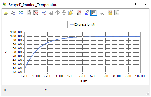
The temperature of the bimetal rises by convection, and the difference in the coefficient of thermal expansion between the metals causes the Helix Coil to bend more. You can see that the inner shaft rotates while winding according to the direction of the coil. After about 7 seconds, most of the external temperature is transmitted and the result converges.

7.3.4.4.3. To view scope expression:

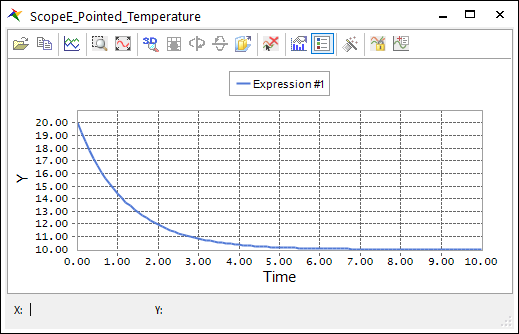
• As shown in the figure below, right-click on ScopeExpression1 created previously in the Database Window, and then click Display.

Check if the input expression result value matches the result checked in Animation.

7.3.4.5. Comparing the results

After applying convection at different temperatures, compare and observe the Animation result and the scope result with the previous ones.

7.3.4.5.1. To modify convection:

1. Right-click Convection1 in the Database Window and click Properties.

2. Change the setting in the Convection dialog as following:

   • Change Ambient Fluid Temperature to 10.

     

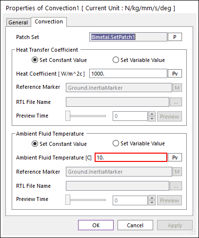
3. Click OK.

7.3.4.5.2. To run simulation:

1. Click the Dynamic/Kinematic Analysis function from the Simulation Type group in the Analysis tab.

2. Change the setting in the General page as following:

   • Output File Name: 10dC

3. Click Simulate.

When the simulation is finished, try again with the changed simulation results for To view the animation and To view scope expression. After that, check whether the ScopeExpression result appears according to the set temperature as shown in the figure below.