4.2. Pendulum Tutorial (CoLink)
4.2.1. Getting Started
4.2.1.1. Objective
In this tutorial, you will simulate and control a dynamic system using CoLink, an interactive environment for designing, simulating, and testing time-varying systems. You will define a control system in CoLink to control a mechanical system that you create in standard RecurDyn.
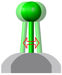
The system to be simulated is a simple inverted pendulum which is mounted on a base which can move side to side. The pendulum can be balanced in its upright position by applying a sideways force to the base. In this tutorial, you will implement various control systems to control this sideways force.
4.2.1.2. Audience
This tutorial is intended for intermediate users of RecurDyn who previously learned how to create geometry, joints, and force entities. All new tasks are explained carefully.
4.2.1.3. Prerequisites
You should first work through the 3D Crank-Slider and Engine with Propeller tutorials, or the equivalent. We assume that you have a basic knowledge of physics.
4.2.1.4. Procedures
The tutorial is comprised of the following procedures. The estimated time to complete each procedure is shown in the table.
Procedures |
Time (minutes) |
Creating the initial model |
10 |
Integrating CoLink |
15 |
Adding Derivative Control |
10 |
Adding Integral Control |
5 |
Total |
40 |
4.2.1.5. Estimated Time to Complete
40 minutes
4.2.2. Creating the Initial Model
4.2.2.1. Task Objective
Learn how to create a mechanical model in preparation for refining the model for use with a control system.
4.2.2.2. Estimated Time to Complete
10 minutes
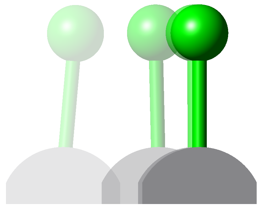
4.2.2.3. Understanding the Model
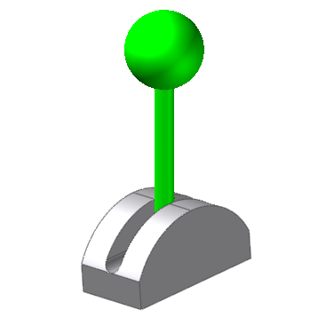
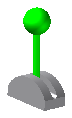
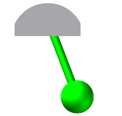
Before starting, the diagram below shows what the completed model should look like.
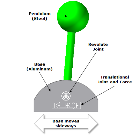
Things to note about the model are:
The pendulum starts offset at a 5-degree angle (from vertical) to perturb the system.
The base is made of aluminum while the pendulum is steel. The appropriate mass densities are already defined in the Parasolid file. You will be able to see the different densities under the Body tab of the Body Properties window after you import the geometry.
The model will be simulated for 5 seconds.
4.2.2.4. Starting RecurDyn and Importing the Geometry
4.2.2.4.1. To start RecurDyn:
On your Desktop, double-click the RecurDyn icon. In the Start RecurDyn window, enter Pendulum as the Model Name.
Click OK.
4.2.2.4.2. To import the geometry:
From the File menu, select Import.
Use the dropdown menu to select ParaSolid File as the file type to import.
Navigate to the CoLink tutorial directory.
- Select the file named invertedPendulum.x_t.(The file path: <InstallDir>\Help\Tutorial\Colink\Pendulum)
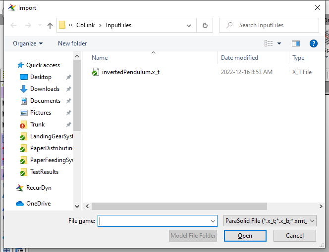
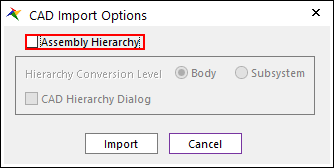
Click Open. The CAD Import Options window appears. Clear the Assembly Hierarchy checkbox and click Import.
Change the Render Mode to Shade. You should now see the two parts of the mechanical model, the inverted pendulum and the base, as shown below.
Select the base and right-click and select Properties.
Under the General page, change the Name to Base.
Click OK.
Repeat steps 7-9 for the pendulum, naming it Pendulum.
4.2.2.5. Adding Joints and Forces
You will now add two mechanical joints and a translational force.
4.2.2.5.1. To add the revolute joint:
From the Joint group in the Professional tab, click the Revolute Joint function.
Set the Creation Method to Body, Body, Point.
Select Base as the base body.
Select Pendulum as the action body.
Enter the point 0, 0, 0 as the joint origin.
From the Database window, right-click on RevJoint1 and select Properties.
Under the Connector page, change the Action Marker’s Euler Angle to -5, 0, 0.
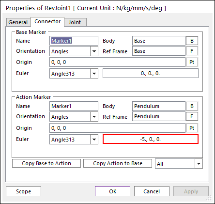
Note
This sets the initial rotational offset of the joint to -5 degrees, which is necessary for the control system to recognize as the starting position.
Click OK.
4.2.2.5.2. To add the translational joint:
From the Joint group in the Professional tab, click the Translational Joint function.
Set the Creation Method to Body, Body, Point, Direction.
Select Ground as the base body.
Select Base as the action body.
Enter the point 0, -50, 0 as the joint origin.
Mouse over the bottom edge of the Base, to the right of the base’s center. The direction of the joint should be indicated as shown at below.
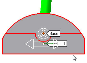
Click on the edge of the Base body.
4.2.2.5.3. To add the translational force:
From the Force group in the Professional tab, click the Translational Force function.
Set the Creation Method to Body, Body, Point, Point.
Select Ground as the base body.
Select Base as the action body.
Enter the point 0, -50, 0 twice, as both the base and action point.
4.2.2.5.4. Save the RecurDyn Model:
Save the Model as Pendulum_P.rdyn.
4.2.2.6. Running a Simulation
You can now run a simulation to see how the uncontrolled pendulum system behaves.
4.2.2.6.1. To run a simulation:
Click the Dynamic/Kinematic Analysis function of the Simulation Type group in the Analysis tab.
Set the simulation to run for 5 seconds with 200 steps as shown in the figure on the below. This will give adequate time to view the motion of the pendulum.
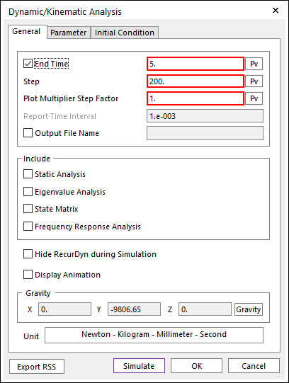
Under the Parameter page, set Numerical Damping to 0.3.
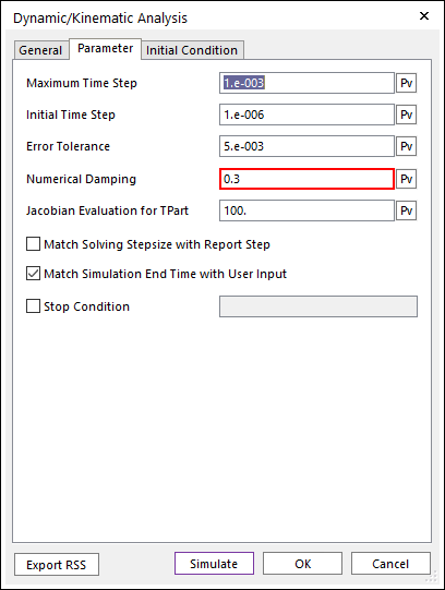
Click Simulate.
4.2.2.7. Viewing the Results
4.2.2.7.1. To view the results:
4.2.2.7.2. Save the RecurDyn Model.
4.2.3. Integrating CoLink
4.2.3.1. Task Objective
In this chapter, you will set up the model for integration with CoLink and create the CoLink model. The CoLink model will be a simple Proportional (P) control system. You will then simulate the controlled system and plot the results.
4.2.3.2. Estimated Time to Complete
15 minutes
4.2.3.3. Creating the General Plant Input
You will first create an input to the model from the control system. This entity will be created as a placeholder that you will then go back and define later.
4.2.3.3.1. To create the General Plant Input:
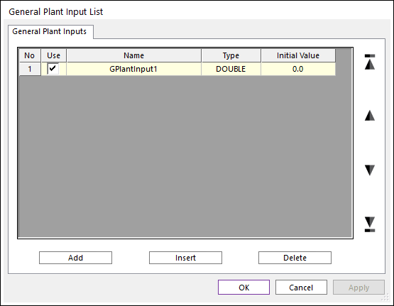
From the GPlant In/Out group in the Communicator tab, click the General Plant Input function.
Click Add.
Click OK.
In the Database Window, right-click on the Translational1 force and select Properties.
Click EL to the right of FX, to define a driving force in the X direction.
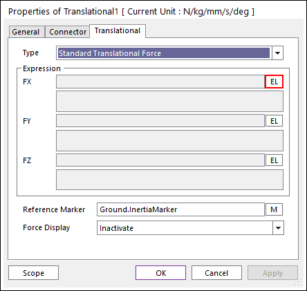
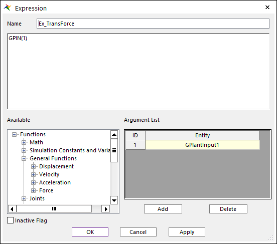
In the Expression List dialog, click Create.
Enter Ex_transForce as the expression Name.
Enter GPIN(1) as the expression.
In the Argument List, click Add.
From the Database Window, drag GPlantInput1 to the first entity of the Argument List as shown in the figure on the below.
Click OK three times to accept all changes.
4.2.3.4. Creating the General Plant Outputs
You will now create an output from the model to the control system. This output will be the pendulum angle, as measured from vertical.
4.2.3.4.1. To create the plant outputs:
Click the General Plant Output function of the Communicator group in the GPlant In/Out tab.
In the General Plant Output List dialog box, click Add.
Click E and Click Create in Expression List.
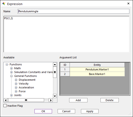
Enter PendulumAngle for Expression name.
Enter PSI(1, 2) as the expression. This expression refers to the PSI angle of the Euler angles to define the rotation between the Pendulum and the Base.
Add two entities to the Argument List and enter the markers that define the Revolute1 joint. Enter the Pendulum marker first, as shown at below.
Click OK twice to accept the changes.
4.2.3.5. Creating the CoLink Model
You will now open CoLink and create the control system. This will involve creating the block diagram from scratch. Blocks will be created to represent the RecurDyn model, gains for a standard P controller, and a scope output.
4.2.3.5.1. To create the CoLink model:
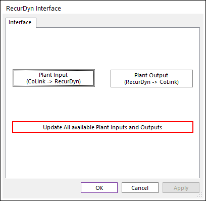
From the CoLink group in the Communicator tab, click the RecurDyn Interface.
In the RecurDyn Interface dialog box, click Update All available Plant Inputs and Outputs.
From the CoLink group in the Communicator tab, click the Run CoLink function. CoLink opens with an empty model.
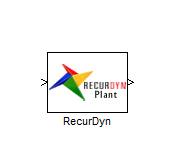
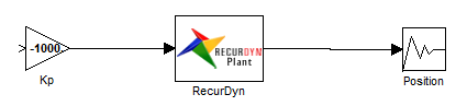
From the Link group in the Connector tab, click the RecurDyn block and then, click into the working window and place it about two thirds of the way to the right as shown below.
From the Output group in the General tab, click the Scope block and then, click into the working window and place it to the right of the RecurDyn block, as shown highlighted in the figure below.
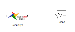
Double-click on the text below the scope block and change the name to Position.
From the Math group in the Math tab, click the Gain block and then, click into the working window and place it to the left of the RecurDyn block, as shown highlighted in the figure below.
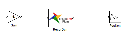
Change the name of the Gain block to Kp by clicking on the name. The vertical text bar will appear.
Double-click on the Gain block to edit the gain value.
Change the Gain to -1000.
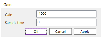
Click OK.
To connect the RecurDyn block to the Position block, as shown below, click the RecurDyn block and hold down Ctrl key and click the Position block. Otherly, click the arrow on the right of the RecurDyn block and drag the cursor to the arrow on the left of the Position block, and then release the mouse button.
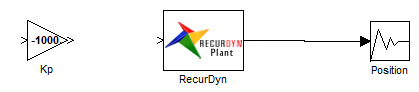
Connect the Kp block to the RecurDyn block.
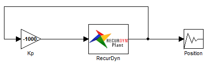
You are now ready to add a proportional control feedback loop that will connect the Position output to the Kp gain block.
4.2.3.5.2. To add a proportional control feedback loop:
Right-click on the line connecting the RecurDyn block to the Position Scope and Drag-Drop to the input of the Kp block.
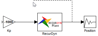
This creates a junction at the point where you first right-clicked. You may need to click on the long horizontal line and drag it up so that it is clear of the other graphics.
4.2.3.5.3. Save the control system:
From the CoLink Quick Access Toolbar, select the Save tool.
Save the CoLink file in the same directory as the RecurDyn model, with the name Pendulum_P.clk.
4.2.3.6. Simulating the CoLink Model
You will now simulate the RecurDyn model with the proportional control system you just created in CoLink.
4.2.3.6.1. To simulate the model with the control system:
The CoLink window does not have a status window. Therefore, before running the simulation you should adjust the location of the CoLink and RecurDyn windows such that you can see the RecurDyn Output window.
From the CoLink Quick Access Toolbar, select the Show Simulation Toolbar menu.
From the Simulation Toolbar, change the simulation end time to 5 seconds, and then change the Type to RecurDyn and change the Solver to RecurDynSolver.

Press the Start function. You should be able to see run status in the RecurDyn Output window.
Tip
What if the co-simulation does not run?
If the co-simulation does not run, a Server Busy dialog box may appear. If the dialog box appears:
Click Switch to and review the message in the RecurDyn Output window.
4.2.3.6.2. To view the results:
Return to the RecurDyn window and press the Play function.
You should see that the pendulum is now kept upright by the control system, oscillating from side to side.
Return to the CoLink window and double-click on the Position scope. You should see a plot of the pendulum’s angular position, as shown at below.
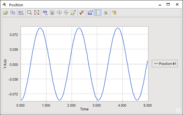
Although the pendulum is kept upright, the plot shows that it oscillates with amplitude that shows little attenuation with time. To remedy this, we will add derivative control in the next chapter.
4.2.4. Adding Derivative Control
4.2.4.1. Task Objective
In this chapter, you will modify the CoLink model to include derivative control, thereby creating a Proportional-Derivative (PD) control system. You will then simulate the system and observe the results.
4.2.4.2. Estimated Time to Complete
10 minutes
4.2.4.3. Modifying the RecurDyn Model
In order to add derivative control, you will first save the RecurDyn model to a different filename, and then modify it to output both pendulum position and velocity (the derivative of position) to the control system.
4.2.4.3.1. To save the model under a different name:
Return to the RecurDyn window.
From the File menu, select the Save As function.
Save the file as Pendulum_PD.rdyn.
4.2.4.3.2. To add a plant output for the rotational velocity of the pendulum:
From the Database window, Right-click on GPlantOutput1 and Select Properties to bring up the General Plant Output List dialog.
Click Add and Click E.
In the Expression List dialog, Click Create.
Enter PendulumAngularVelocity and Enter WZ(1, 2) for the expression.
Add the same two markers as before to the Argument List, as shown at below.
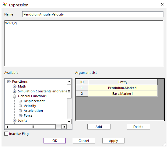
Click OK three times to accept the changes.
From the CoLink group in the Communicator tab, click the RecurDyn Interface function.
In the RecurDyn Interface dialog box, click Update All available Plant Inputs and Outputs.
4.2.4.4. Adding Derivative Control
You will first save the CoLink model to a different filename, and then modify it to include another feedback loop which will handle derivative control.
4.2.4.4.1. To save the control system under a different name:
Return to the CoLink window.
From the File menu, select the Save As tool.
Save the file as Pendulum_PD.clk.
4.2.4.4.2. To add derivative control:
Delete all of the connections between the blocks by selecting them and then pressing the Delete key.
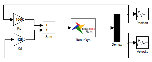
Use the figure to guide you through the next steps:
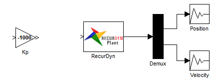
From the Connector group in the Connector tab, click the Demux block and then, click into the working window. Place it between the RecurDyn block and the Position scope.
Add another Scope (Output) below the Position scope.
Rename the scope to Velocity.
Make connections between the RecurDyn plant, the Demux block, and the Position and Velocity scopes according to the diagram.
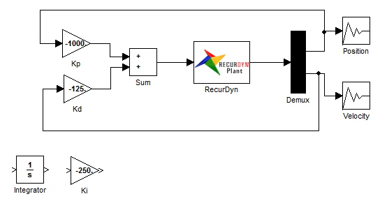
Add another gain block below the Kp gain block, as shown below.
Rename the new gain block Kd.
Change the gain value to -125.
From the Math group in the Math tab, click the Sum block and then, click into the working window. Place it between the Kp gain block and the RecurDyn plant.
Make connections between the gain blocks, the sum block, and the RecurDyn plant according to the diagram below.
Press the Start function. You should be able to see run status in the RecurDyn Output window.
Save the control system.
4.2.4.5. Simulating the Model with Derivative Control
4.2.4.5.1. Simulate the model as before
Tip
What if the Run arrow is grayed out?
On rare occasions the CoLink Run arrow stays grayed out. If that happens, simply save the CoLink model, close CoLink, restart CoLink and reload the model.
4.2.4.5.2. To view the results:
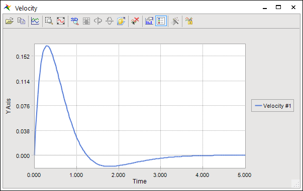
Double-click on the Position and Velocity scopes. You should see the following results:
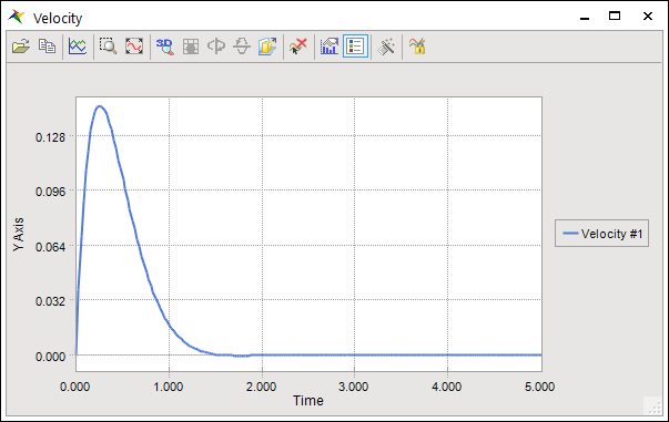
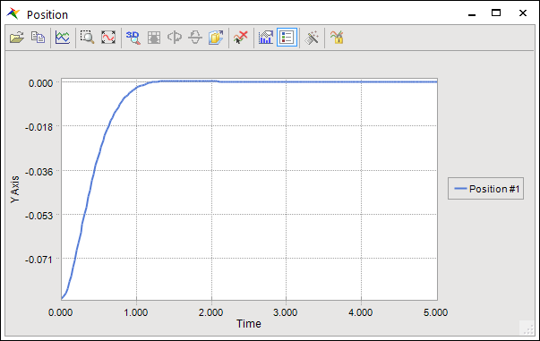
It appears that the results are much better, as both the angular position and velocity of the pendulum now converge to zero, instead of oscillating.
Return to the RecurDyn window.
Play the animation.
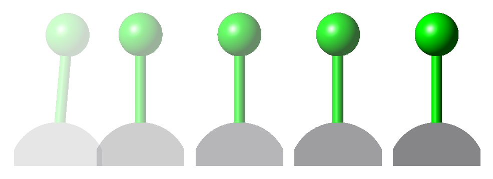
The animation shows that while the pendulum indeed stays upright, the entire system drifts off to the right. To reduce the drifting, you will add integral control in the next chapter.
4.2.5. Adding Integral Control
4.2.5.1. Task Objective
In this chapter, you will modify the CoLink model to include integral control, thereby creating a Proportional-Integral-Derivative (PID) control system. You will then simulate the system and observe the results.
4.2.5.2. Estimated Time to Complete
5 minutes
4.2.5.3. Adding Integral Control
You will first save the CoLink model to a different filename, and then modify it to include another feedback loop which will handle integral control.
4.2.5.3.1. To save the control system under a different name:
From the CoLink File menu, select the Save As tool.
Save the file as Pendulum_PID.clk.
4.2.5.3.2. To add derivative control:
Double-click on the Sum block.
Enter +++ for the List of signs. This will increase the number of inputs to the Sum block to three.
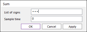
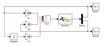
Click OK. Use the figure below to guide you through the next steps:
From the Continuous group in the Continuous and Discrete tab, click the Integrator block and then, click into the working window. Place it below and to the left of the Kd gain block.
Place another gain block in the model, below the Kd gain block.
Name the gain block Ki.
Change the gain value to -250.
Make the three connections shown below in red.
Press the Start funciton. You should be able to see run status in the RecurDyn Output window.
Save the control system.
4.2.5.4. Simulating the Model with PID Control
4.2.5.4.1. Simulate the model as before
4.2.5.4.2. To view the results:
Double-click on the Position and Velocity scopes. You should see the following results:
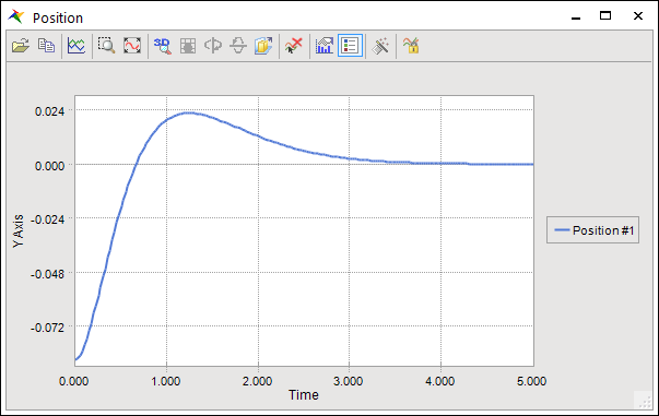
There is now some overshoot in the positional response as it converges to zero.
Return to the RecurDyn window.
Play the animation.
The animation now shows that the pendulum stays upright, and the base comes to a near stop instead of sliding away as before. Therefore, with the addition of more types of control feedback loops, the control system becomes more adept at stabilizing the system.