1.3. Pinball Tutorial (Professional)

1.3.1. Getting Started

1.3.1.1. Objective

The modeling and simulation of contact between bodies are important topics in multibody dynamics. RecurDyn has powerful capabilities to define and simulate all types of contacts, from simple to complex and with body geometry created in RecurDyn, as well as geometry that is imported from CAD software. Consideration of contacts is needed to model designs that have interesting responses to model changes.

In this tutorial, you will act as a company developing a novel pinball machine that includes a higher level of vertical motion. One aspect of the model is that the ball goes up and down a curved ramp as it is propelled from its starting point. The purpose of the tutorial is to select the spring that can store sufficient energy to propel the ball over the vertical obstacle.

This tutorial provides the first exposure to the modeling. You will learn about below.

• Create geometry.

• Define contacts between bodies.

• Define a parametric value.

• Run a design study.

You will also learn below.

• Simulate a small portion of a pinball game, where balls contact with each other and guides that act as boundaries.

• Study the relationship between the driving force of the ball launcher and the response of the system.

1.3.1.2. Audience

This tutorial is intended for new users of RecurDyn. All new tasks are explained carefully.

1.3.1.3. Prerequisites

Users should firstly work through the 3D Crank-Slider Tutorial and the Engine with Propeller Tutorial, or the equivalent. We assume that you have a basic knowledge of physics.

1.3.1.4. Procedures

The tutorial is comprised of the following procedures. The estimated time to complete each procedure is shown in the table.

Procedures	Time (minutes)
Setting Up Your Simulation Environment	5
Creating Geometry	5
Creating Force and Contact	15
Creating Expression Scope and PerformingAnalysis	10
Performing a Design Study	30
Total	65

1.3.1.5. Estimated Time to Complete

65 minutes

1.3.2. Setting Up Your Simulation

1.3.2.1. Task Objective

Learn how to set up the simulation environment, including units, materials, gravity, and the working plane.

1.3.2.2. Estimated Time to Complete

5 minutes

1.3.2.3. Starting RecurDyn

1.3.2.3.1. To start RecurDyn and create a new model

1. On your Desktop, double-click the RecurDyn icon. RecurDyn starts and the Start RecurDyn window appears.

   

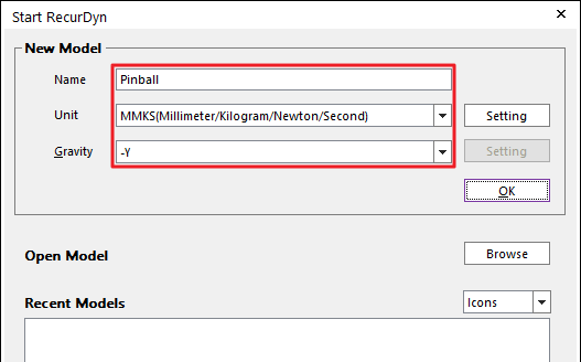
2. Enter the name of the new model as Pinball.

3. Change Unit to MMKS.

4. Change Gravity to -Y.

5. Click OK.

1.3.2.4. Adjusting the Icon and Marker Size

You are now going to change the icon and marker size to 10 pixels so you can view the model better.

1.3.2.4.1. To change the icon and marker size

1. In the Render Toolbar, click the Icon Control tool. The Icon Control window appears.

2. Set Icon Size and Marker Size to 10.

   

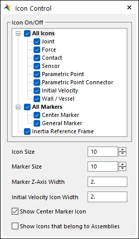
3. Close Icon Control window.

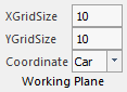
1.3.2.4.2. To set the grid size to 10

From the Working Plane group in the Home tab, set the grid size to 10 in both text boxes by placing the cursor in each text box, and then pressing the Enter key.

1.3.3. Creating Geometry

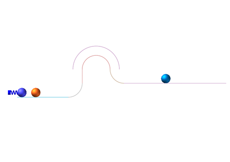
You will use wireframe geometry to define the ball guides in this pinball model. You will define all of the guides on the ground body and define several balls at the model level as individual bodies.

1.3.3.1. Task Objective

Learn to create:

• Line and arc geometry that will guide the motion of the balls.

• Spherical geometry that represents the three balls in the model.

• Circle geometry inside ball for 2D Contact between circle and guide.

1.3.3.2. Estimated Time to Complete

10 minutes

1.3.3.3. Creating the Guide Geometry

1.3.3.3.1. To create the straight guide geometry

1. To enter Body Edit Mode for the Ground body, from the Body group in the Professional tab, click the Ground function.

   You know that RecurDyn is in Body Edit Mode for the Ground body because

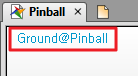
   • The title in the upper left corner of the working model window changes to Ground@Pinball.

     

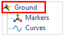
   • The top item in the database window is Ground.

     

2. Change the working plane to the XY Plane.

3. From the Curve group in the Ground tab, click the Outline function.

4. Set the Creation Method to MultiPoint.

   • Point 1: 0, 0, 0

   • Point 2: 110, 0, 0

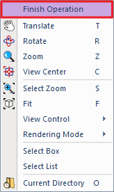
5. Right-click and then click Finish Operation (the top item in the menu that appears) to finish the definition of the outline.

   

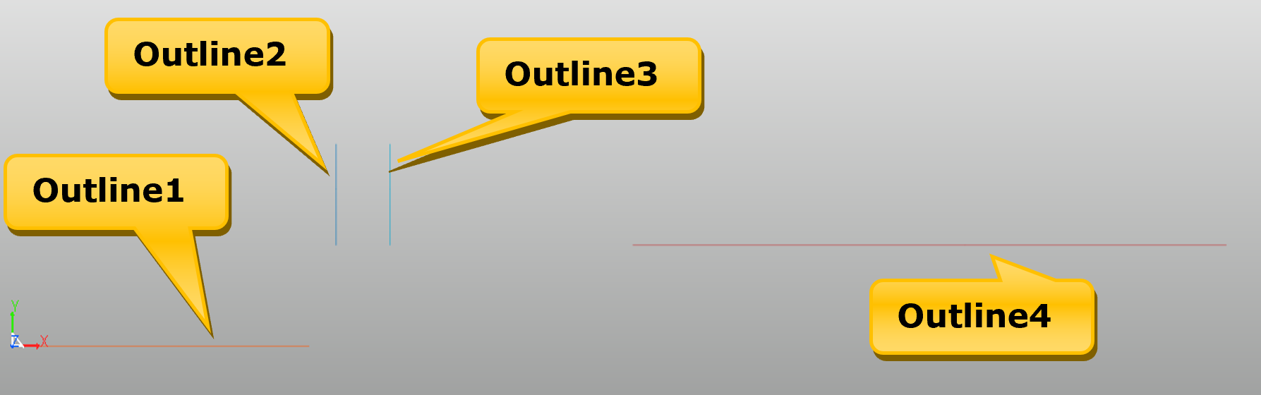
6. Repeat Steps 3-5 three times using following information.

   • Point 1: 120, 30, 0

   • Point 2: 120, 60, 0

   • Point 1: 140, 30, 0

   • Point 2: 140, 60, 0

   • Point 1: 230, 30, 0

   • Point 2: 450, 30, 0

   The following appears in the working model window.

   

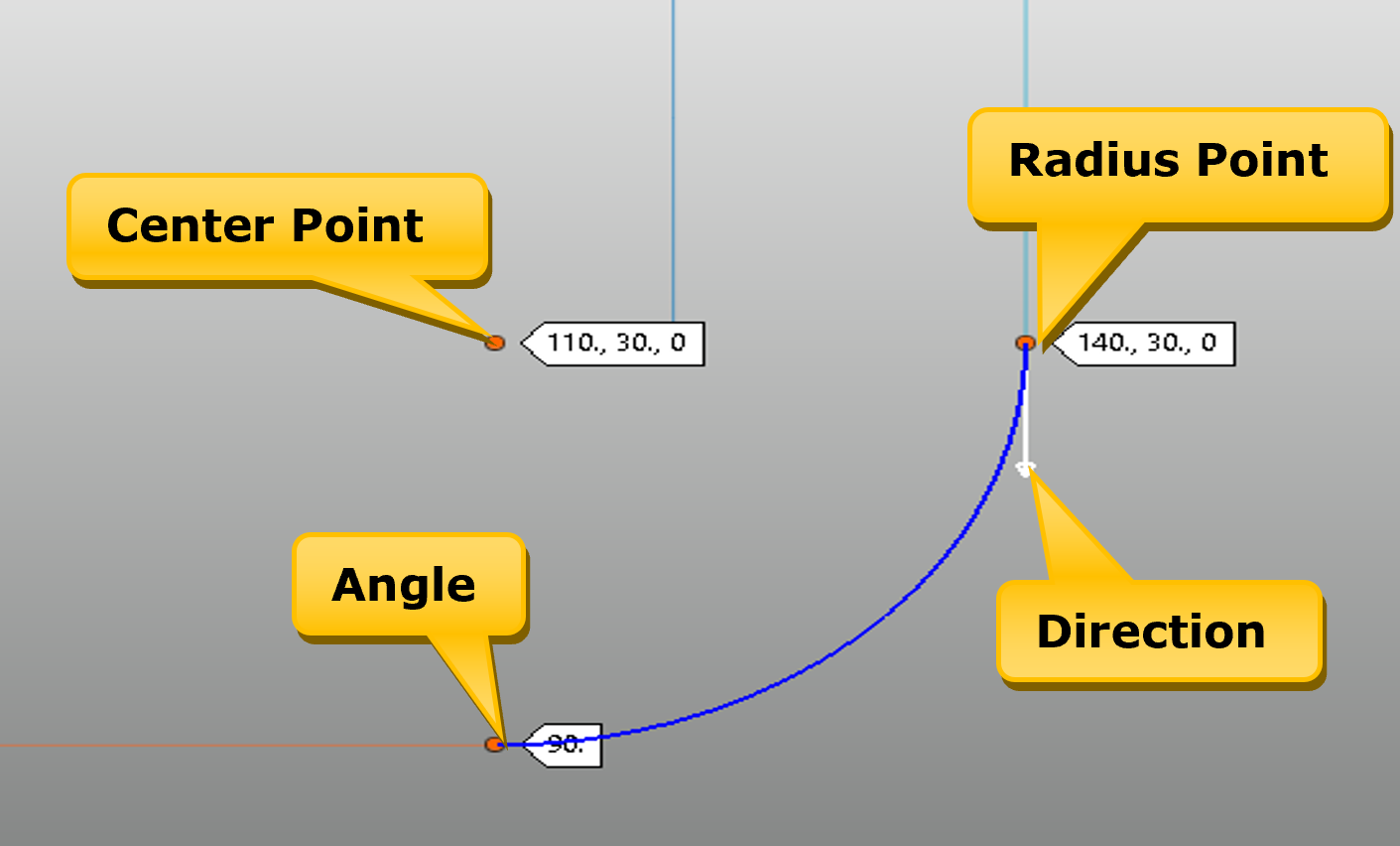
1.3.3.3.2. To create the arc guide geometry

1. From the Curve group in the Ground tab, click the Arc function.

2. Set the Creation Method to Point, Point, Direction, Angle.

   • Center Point: 110, 30, 0

   • Radius Point: 140, 30, 0

   • Direction: 0, -1, 0

   • Angle: 90

   

3. Repeat Steps 1-2 three times using following information.

   • Center Point: 170, 60, 0

   • Radius Point: 140, 60, 0

   • Direction: 0, 1, 0

   • Angle: 180

   • Center Point: 170, 60, 0

   • Radius Point: 120, 60, 0

   • Direction: 0, 1, 0

   • Angle: 180

   • Center Point: 230, 60, 0

   • Radius Point: 200, 60, 0

   • Direction: 0, -1, 0

   • Angle: 90

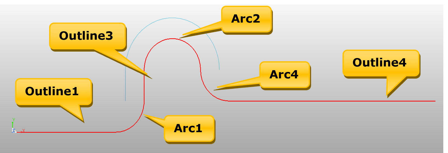
   The geometry appears as shown in the figure below.

   

1.3.3.3.3. To create EdgeCurve geometry with existing curves

1. From the Curve group in the Ground tab, click the Edge Curve function.

2. Set the Creation Method to MultiEdge.

3. Use the Select Toolbar to curves except Outline2 and Arc3 as shown in the figure below.

   

   Tip

   Use Select Toolbar to easily select Multi Edges

   

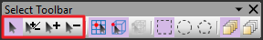
   You can change Select State of mouse cursor with Select Toolbar.

   • Select(Default): It clears already selected entities when selecting new entities.

   • Add or Remove: Reverse Select State of already selected entities. When selecting entities, it deselects already selected entities and selects deselected entities.

   • Add: It keeps already selected entities and can only add other entity newly.

   • Remove: It only deselect selected entities.

   Other functions in Select Toolbar will vary with different Edit Modes.

4. When you select all the curves in lower part, right-click on working window and click Finish Operation.

5. From the Curve group in the Ground tab, click the Edge Curve function again.

6. Set the Creation Method to MultiEdge.

7. Use the Select Toolbar to Outline2 and Arc3 as shown in the figure below.

   

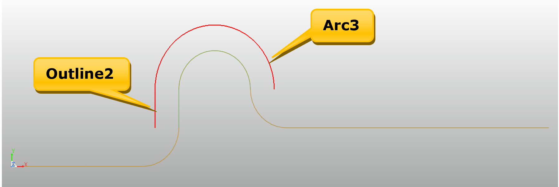
8. When you select all the curves in lower part, right-click on working window and click Finish Operation.

9. Delete all other curves except EdgeCurve1 and EdgeCurve2.

   

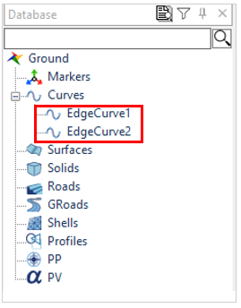
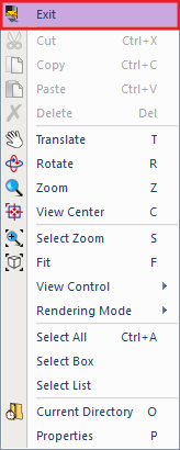
10. Click Exit to exit the body edit mode. (Exit button is in Ribbon Menu, it is also in right-click menu when you right-click on Working Window.)

    

1.3.3.4. Creating the Ball Geometry

1.3.3.4.1. To create the Ball geometry and Circle Geometry

1. From the Marker and Body group in the Professional tab, click the Ellipsoid function.

2. Set the Creation Method to Point, Distance.

   • Point: 10, 10, 0

   • Distance: 10

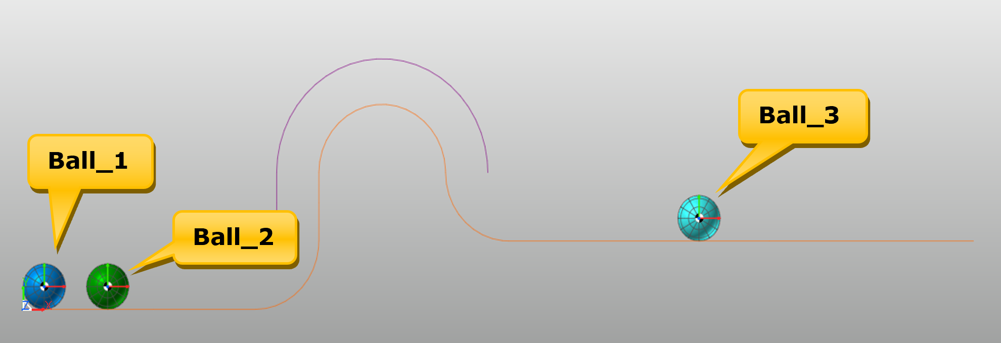
3. Open the properties dialog and rename the Body1 to Ball_1.

4. Repeat Steps 1-3 twice using following information.

   • Point: 40, 10, 0

   • Distance: 10

   • Body Name: Ball_2

   • Point: 320, 40, 0

   • Distance: 10

   • Body Name: Ball_3

1.3.3.5. Saving the Model

Take a moment to save your model before you continue with the next chapter.

• From the File menu, click the Save function.

1.3.4. Creating Force and Contact

The behavior of this model is driven by forces. A compressed spring drives Ball_1 into Ball_2. The continuing motion of the balls results from gravity forces, contacts between balls, and contacts between the balls and the geometry.

1.3.4.1. Task Objective

Learn to create three types of force elements:

• Compressed spring that will act on Ball_1

• Sphere To Sphere contacts between the balls

• Geo Curve contacts between the balls and the Guides.

1.3.4.2. Estimated Time to Complete

20 minutes

1.3.4.3. Defining the Compressed Spring

You will create a spring force and adjust its properties to reflect that it is a compressed spring. As a result, Ball_1 will be pushed to the right when the simulation begins.

1.3.4.3.1. To create the spring

1. From the Force group in the Professional tab, click the Spring Force function.

2. Set the Creation Method to Body, Body, Point, Point.

3. Click in the background of the Working window to select the Ground body to be the base body of the Spring.

4. Click on the Ball_1 geometry to select Ball_1 to be the action body of the Spring.

5. Click on the following locations in the Working window.

   • Point1: -20, 10, 0

   • Point2: 10, 10, 0

1.3.4.3.2. To adjust the spring properties

1. Display the Properties window for the spring, which will have the name of Spring1.

2. In the Spring page, change.

   • Stiffness Coefficient: 20

   • Damping Coefficient: 0.05

   • Free Length: 45

     

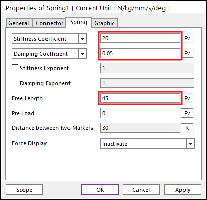
   The length as defined is 30 mm. By changing the Free Length to 45, you are indicating that the spring is compressed by 15 mm. Given the spring Coefficient of 10, a load of 150 N will be applied to the ball at the beginning of the simulation. Once the spring length increases to 45 mm, the force becomes zero.

3. In the Graphic page, change the spring diameter value to 10.

   

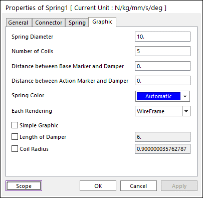
4. Click OK.

1.3.4.4. Defining the Contact between the Balls

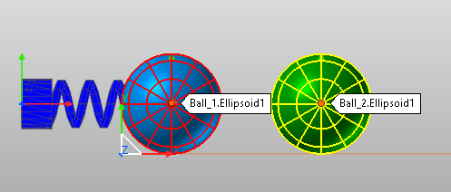
1.3.4.4.1. To create the contact between the balls

1. From the Contact group in the Professional tab, click the Sphere to Sphere Contact function.

2. Set the Creation Method to Sphere, Sphere.

3. Select the following geometries.

   • Sphere: Ball_1.Ellipsoid1

   • Sphere: Ball_2.Ellipsoid1

   

4. From the Contact group in the Professional tab, click the Sphere to Sphere Contact function and select the following geometries.

   • Sphere: Ball_2.Ellipsoid1

   • Sphere: Ball_3.Ellipsoid1

1.3.4.4.2. To adjust the contact between the balls

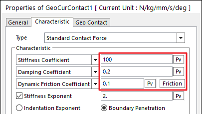
1. Open the Properties dialog of SphereToSphere1.

2. In the Characteristics page, change:

   • Stiffness Coefficient: 100

   • Damping Coefficient: 0.2

   • Dynamic Friction Coefficient: 0.1

     

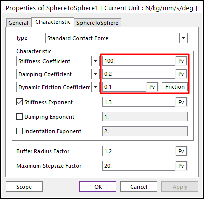
3. Click OK.

4. Change the SphereToSphere2 Properties with same settings above.

1.3.4.5. Defining Contact Between the Balls and Guides

The first ball (Ball_1) is constrained by the spring and will only contact the straight line as the left of the guide geometry.

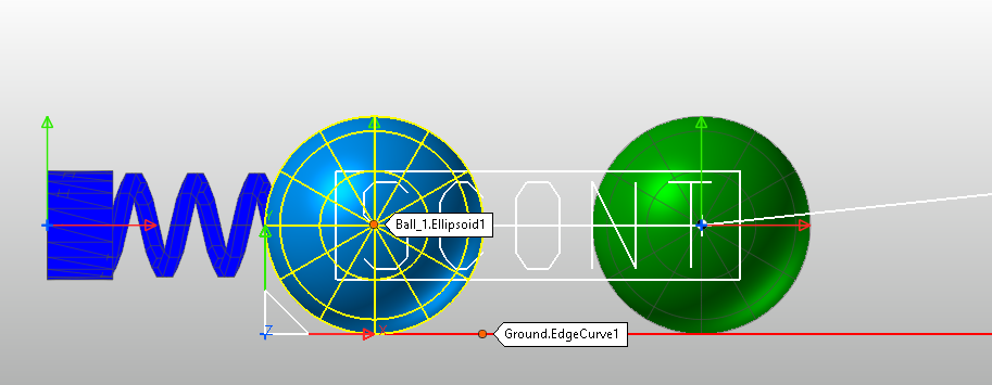
1.3.4.5.1. To create the contact between the first ball (Ball_1) and the guide geometry

1. From the 2D Contact group in the Professional tab, click the Geo Circle Contact function and select geometries below.

   • Curve: Ground.EdgeCurve1

   • Circle(Sphere): Ball_1.Ellipsoid1

   

2. Open the Properties dialog of GeoCurContact1.

3. In Geo Contact page, change the normal directions in Preview as shown below.

   • Contact Plane Normal(Base/Action): 0, 0, 1

   • Normal Direction(Base): Up

     

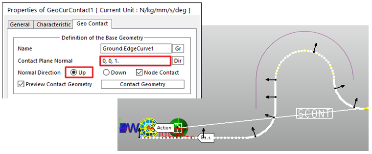
4. In the Characteristics page, change.

   • Stiffness Coefficient: 100

   • Damping Coefficient: 0.2

   • Dynamic Friction Coefficient: 0.1

     

5. Click OK.

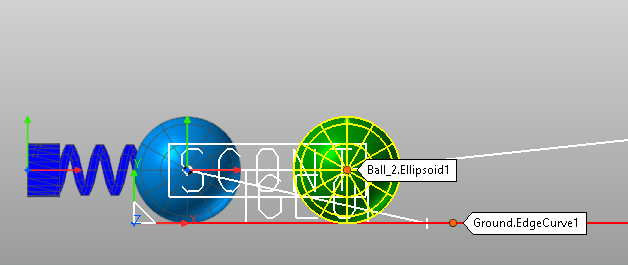
1.3.4.5.2. To create the contact between the second ball (Ball_2) and the guide geometry

1. From the 2D Contact group in the Professional tab, click the Geo Circle Contact function and select following geometries.

   • Curve: Ground.EdgeCurve1

   • Circle(Sphere): Ball_2.Ellipsoid1

   

2. Open the Properties dialog of GeoCurContact2.

3. In Geo Contact page, change the normal directions in Preview as shown below.

   • Contact Plane Normal(Base): 0, 0, 1

   • Normal Direction(Base): Up

     

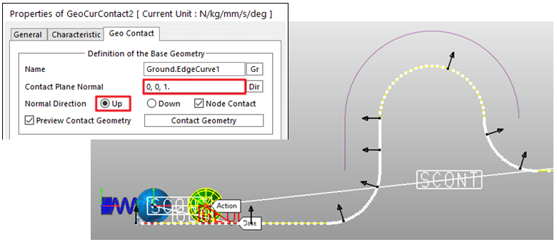
4. In the Characteristics page, change.

   • Stiffness Coefficient: 100

   • Damping Coefficient: 0.2

   • Dynamic Friction Coefficient: 0.03

5. Click OK.

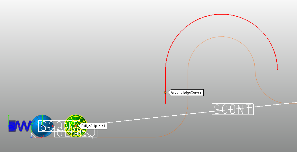
1.3.4.5.3. To create the contact between the Ball_2 and the arc Guide geometry

1. From the 2D Contact group in the Professional tab, click the Geo Circle Contact function and select following geometries.

   • Curve: Ground.EdgeCurve2

   • Circle: Ball_2.Ellipsoid1

   

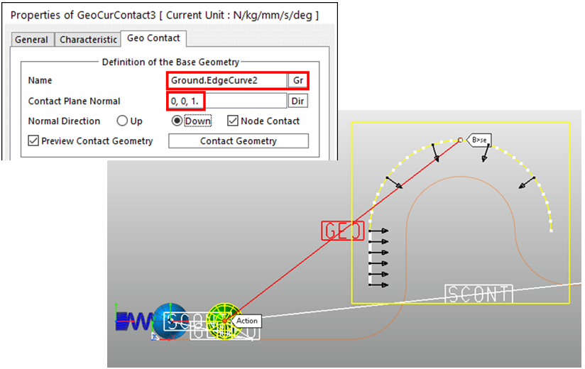
2. Open the Properties dialog of GeoCurContact3.

3. In Geo Contact page, change the normal directions in Preview into the following configurations as shown below.

   • Contact Plane Normal(Base): 0, 0, 1

   • Normal Direction(Base): Down

     

4. In the Characteristics page, change.

   • Stiffness Coefficient: 100

   • Damping Coefficient: 0.2

   • Dynamic Friction Coefficient: 0.03

5. Click OK.

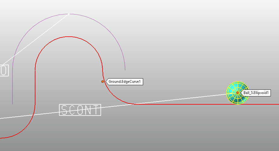
1.3.4.5.4. To create the contact between the Ball_3 and the lower Guide geometry

1. From the 2D Contact group in the Professional tab, click the Geo Circle Contact function and select following geometries.

   • Curve: Ground.EdgeCurve1

   • Circle(Sphere): Ball_3.Ellipsoid1

   

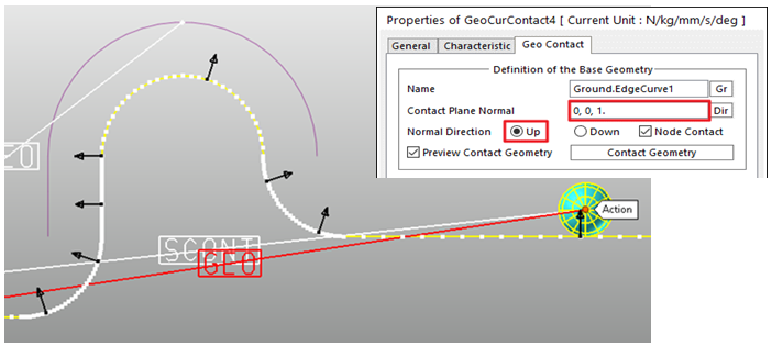
2. Open the Properties dialog of GeoCurContact4.

3. In Geo Contact page, change the normal directions in Preview into the following configurations as shown below.

   • Contact Plane Normal(Base): 0, 0, 1

   • Normal Direction(Base): Up

   

4. In the Characteristics page, change.

   • Stiffness Coefficient: 100

   • Damping Coefficient: 0.2

   • Dynamic Friction Coefficient: 0.1

5. Click OK.

1.3.4.5.5. To define the Smooth Node Contact and define force displays

Set the additional options to make smooth contact between guides and balls and define Force Display options for the visualization of Contact Forces in animation.

1. From GeoCurContact1 to GeoCurContact4, select 4 Contacts from Database. Then right-click holding Ctrl key to click Properties.

   

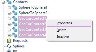
   Multi-Properties dialog is shown which can change the properties of selected entities.

2. In Geo Contact page, Uncheck Node Contact of Base Geometry.

   

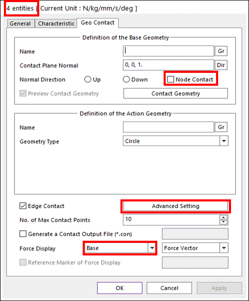
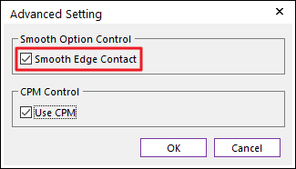
3. In Geo Contact page, click Advanced Setting.

4. In Advanced Setting dialog, check on the Smooth Edge Contact option and click OK.

   

5. In Geo Contact page, change Force Display to Base.

6. Click OK in Multi-Properties dialog.

1.3.4.6. Saving the Model

Take a moment to save your model before you continue with the next chapter.

• Click the Save function in File menu.

1.3.5. Creating Expression Scope

1.3.5.1. Task Objective

In this chapter, you’ll run a simulation of the model you just created. Furthermore, you will define the expression measuring the distance between two bodies and run the simulation. Also, you will monitor the expression result through the scope.

1.3.5.2. Estimated Time to Complete

30 minutes

1.3.5.3. Defining Expression

You will define the expression measuring distance between two bodies.

1. From the Expression group in the SubEntity tab, click the Expression function. The Expression List dialog will appear.

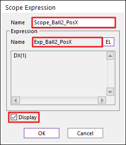
2. Click Create. The Expression dialog will appear.

3. Change Name to Exp_Ball2_PosX. Enter the following expression in the large text box: DX(1)

4. Click Add located below Argument List.

5. In the Database window, click + in front of Ball_2 and Markers.

6. Drag CM in Ball_2 markers and drop in empty text box in the Argument List.

   

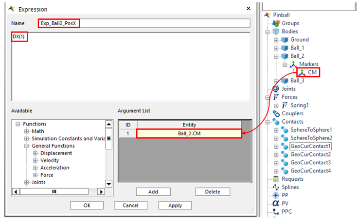
7. Click OK in the Expression dialog.

8. Click OK in the Expression List dialog.

Tip

Changing Markers in Expression

In the above Expression, the Center Marker (CM) used in the Argument List means the marker of the mass center of the body. You can use the General Marker which you can define instead of CM in Expression.

You can create the General Marker by clicking Marker from the Marker and Body group in the Professional Tab.

1.3.5.4. Creating Expression Scope

You can monitor the result of Exp_Ball2_PosX with Scope without going through Plot.

1. From the Scope group in the Analysis tab, Click the Expression Scope function.

2. Change Name to Scope_Ball2_PosX.

3. Click EL button to select Exp_Ball2_PosX and Click OK.

4. Check Display and Click OK.

   

Now you are ready to monitor the Scope of Expression.

1.3.5.5. Performing Dynamic/Kinematic Analysis

In this section, you will run a dynamic/kinematic analysis to view the effect of forces and motion on the model you just created.

1.3.5.5.1. To perform a dynamic/kinematic analysis

1. From the Simulation Type group in the Analysis tab, click the Dynamic / Kinematic Analysis function.

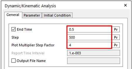
2. In the General page, define the end time of the simulation and the number of steps:

   • End Time: 0.5

   • Step: 500

   • Plot Multiplier Step Factor: 4

     

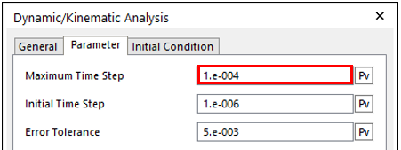
3. In the Parameter page, define the Maximum Time Step to 1.e-004.

   

4. Click Simulate.

   RecurDyn calculates the motions and forces in the balls, spring and contacts. There will be 2000 plot outputs stored because the Number of Steps is 500 and the Plot Multiplier Step Factor is 4.

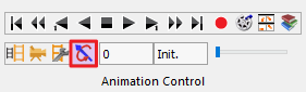
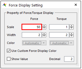
5. From the Animation Control group in Analysis tab, click the Force Display Setting function.

   

6. Change Scale to 50 to clearly monitor the Force Display result of Contact.

   

7. In Render Toolbar, click the Icon Control tool.

8. Uncheck All Icons to disappear the icons on Working Window.

   

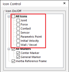
9. Close Icon Control window.

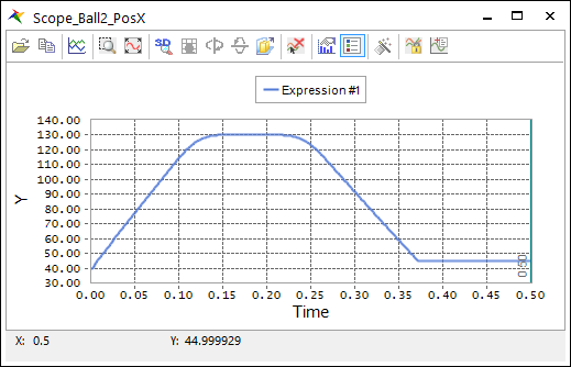
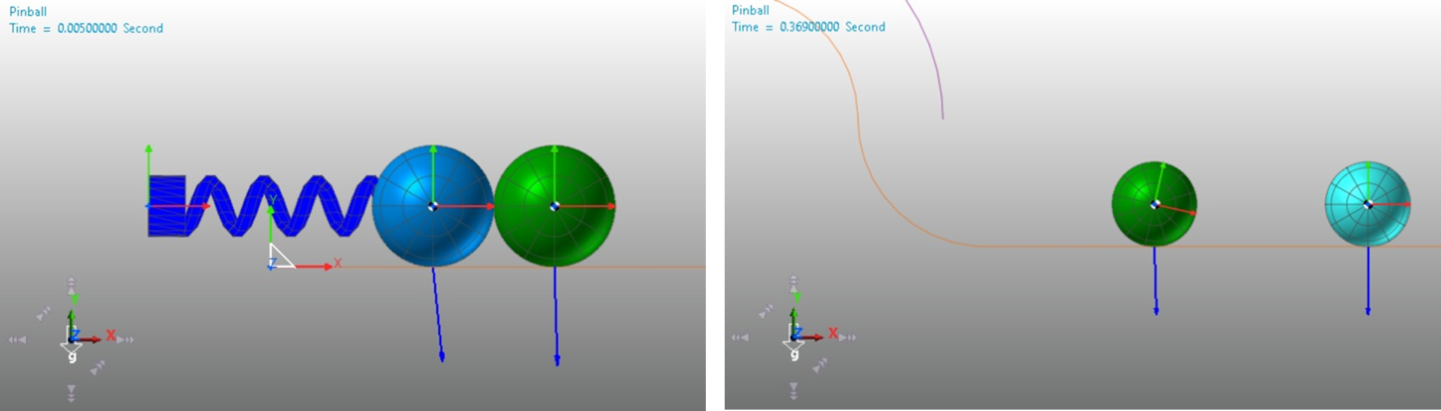
10. From Animation Control group in Analysis tab, click the Play function to play the animation.

    

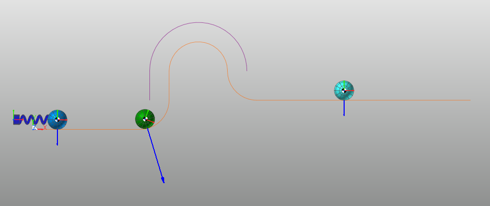
You will see the result of Expression Scope as shown below.

You look in the spring catalog and you find that this spring is available in 1 mm increments from 45 mm through 54m. You want to try out different lengths of the spring, but you don’t want to have run the various cases and keep track of the results manually.

You want to do an automated design study, which is explained in next chapter.

1.3.6. Performing a Design Study

1.3.6.1. Task Objective

In this chapter, you will rerun the simulation under a design study environment to decide how to select a spring that will provide the right energy to move the ball over the hump.

1.3.6.2. Estimated Time to Complete

30 minutes

1.3.6.3. Performing a Design Study

The steps to performing a design study for this model are below.

1. Define the free length of the spring as a Parametric Value that can be adjusted during the design study.

2. Define a Design Variable from the Parametric Value, where you add information about the data boundaries. The range of the free length of the spring is from 45 to 54 mm.

3. Define a Performance Index. This is an outcome of interest for the design study.

   In this case, you will measure the maximum position of Ball_2 in the X direction. If the maximum position of Ball_2 is more than 170, then you know that it has passed the top of the vertical obstacle.

4. Set the Number of Trials for this design study, which is 10.

5. Run the DOE. Outputs will automatically be directed to different output files.

6. Review and Plot the results from the DOE.

7. Animate a particular trial.

1.3.6.3.1. To define a parametric value

1. Display the Properties window for the Spring1.

2. Next to the Free Length text box, click PV.

3. When the Parametric Value List window appears, click the Add button and change like as below.

   • Name: Spring_Free_Length.

   • Value: 45

     

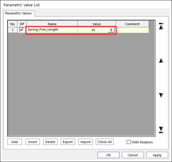
4. Click OK to exit the Parametric Value List window.

5. Click OK to exit the Spring1 Properties window. You will see that the name of the Parametric Value appears in the Free Length text box.

1.3.6.3.2. To define a design variable:

1. Click the Design Variable function from the Design Study group in the Subentity tab. The Design Variable List window appears.

2. In the Design Variable List window, click the Create button. The Design Variable window appears.

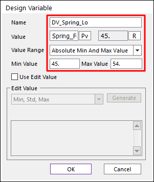
3. Do the following in the window:

   • Name: DV_Spring_Lo.

   • Value: Spring_Free_Length

   • Value Range: Absolute Min And Max Value

   • Min Value: 45

   • Max Value: 54

     

4. Click OK to exit the Design Variable window.

5. Click OK to exit the Design Variable List window.

1.3.6.3.3. To define a performance Index

1. Click the Performance Index function from the Design Study group in the Subentity tab. The Performance Index List window appears.

2. Set the Type at the bottom left to Expression and Click Add in the Performance Index List window.

   • Name: Ball_2_Travel

   • Result Output: Exp_Ball2_PosX

   • Treatment: Max Value

     

3. Click OK.

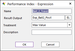
4. Click OK to exit the Performance Index List window.

1.3.6.3.4. To set the number of trials

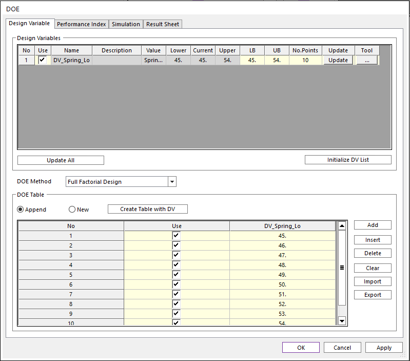
1. Click the Design Study function from the Simulation Type group in the Analysis tab. The DOE window appears.

2. Change 10 in Number of Points of DV_Spring_Lo and Click Update In the DOE window.

3. Click the Create Table with DV button and you will see 10 Trials created as shown below.

   

1.3.6.3.5. To run the design study

1. In the DOE window, click the Simulation page.

2. Click to R-Button in Number of Trials and you can see that it is updated to 10.

3. Click Simulate. 10 runs occur in the output window. When the runs are complete, the Design Study window reappears.

1.3.6.3.6. To review and plot results

1. Click the Result Sheet page.

   A list of the 10 runs appears:

   • The first column displays the value of the Free Length of the spring.

   • The second column displays the maximum X value of the center of Ball_2.

   

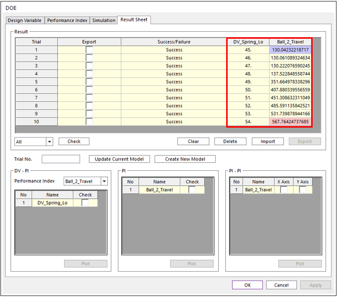
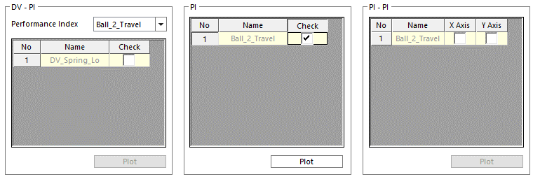
2. To plot the Ball_2_Travel Performance Index, under the PI heading, click the box in Ball_2_Travel, and then click Plot.

   

3. The following plot appears when you click Plot.

   

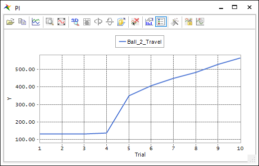
4. Click the x in the upper right corner and to close the plot and click OK in the DOE window.

1.3.6.4. Animating the Results of a Trial

You’ll first take a look at Trial 6, which is the firstly trial where Ball_2 makes it over the vertical obstacle.

1.3.6.4.1. To animate the results of a particular trial:

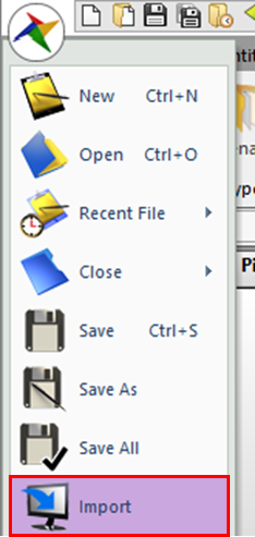
1. From the File menu, click the Import function.

   

2. Set Files of type to RecurDyn Animation Data File (*.rad).

3. Double-click Pinball_6.rad, which contains the animation results for Trial 6.

4. Animate the model using the Play tool on the Animation Toolbar.

1.3.6.4.2. To animate the result using select camera

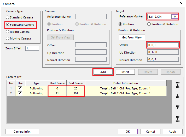
1. From the Animation Control group in the Analysis tab, click the Select Camera function. The Camera window appears.

2. In Camera Type section, Select Following Camera.

3. In Target section, enter the following information.

   • Reference Marker: Ball_1.CM

   • Offset: 0, 0, 0

4. Click Add to add camera. Enter the following information in the Camera List.

   • Start Frame: 0

   • End Frame: 20

5. Repeat Steps 2-4 twice using following information:

   • Reference Marker: Ball_2.CM

   • Offset: 0, 0, 0

   • Start Frame: 21

   • End Frame: 501

     

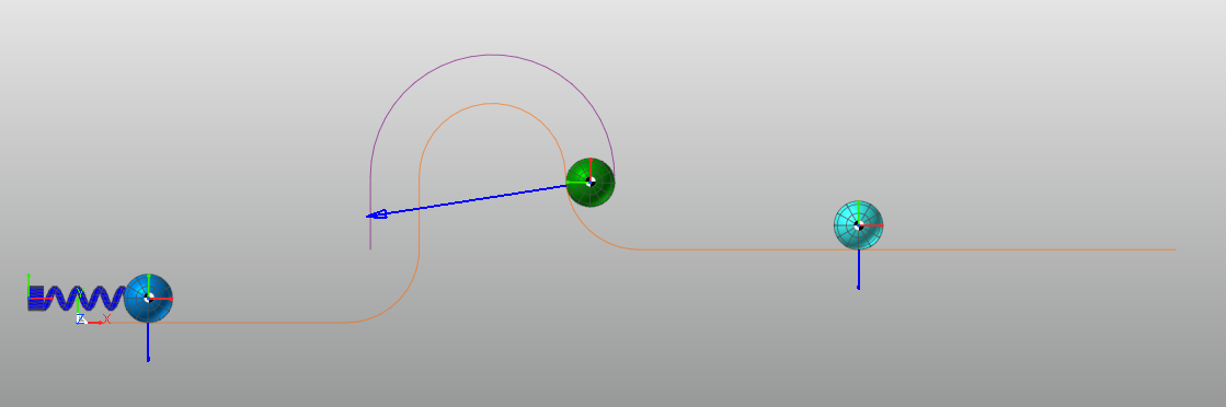
From 0 to 20 frame, camera follows Ball_1_CM and from 21 to 501 frame, camera follows the Ball_2_CM as shown below. You can do better posting if you set up with other Camera Types on your desired frames.

1.3.6.5. Ideas for Further Exploration

You can gain a good understanding of the behavior of the pinball model by looking at the animations through several trials. Here are more things to consider:

• The model used a low coefficient of friction (0.1). It represents the friction of a polished steel ball contacting with a smooth, dry surface. Low friction is a good assumption for the new pinball machine, but what if when the machine becomes old (by a dirt and some corrosion)?

  • How will results be changed when the friction coefficient is changed?

  • What could you do to study the effects of increased friction in this model?

  • Does increased friction require a stronger or weaker spring?