1.4. Ball Return Tutorial (Professional)

1.4.1. Getting Started

1.4.1.1. Objective

The modeling and simulation of contact between bodies are important topics in multibody dynamics. RecurDyn has powerful capabilities to define and simulate 3D contacts. The example in this tutorial is to model a bowling ball return system and the container that collects the balls.

In this tutorial, you learn how to generate 3D contacts with enough detail to be able to model sophisticated contacts on your own. For simple demonstrations, it may seem appealing to simply define complete body-to-body contact. Real models, however, are often too complex to simulate efficiently when every possible contact is considered. RecurDyn offers the powerful capability to select faces to create logical contact surfaces. When you define the contacts, you can then use the logical contact surfaces. Then you can do contact modeling effectively.

This tutorial provides an introduction to 3D contact modeling by using imported geometry. You will learn how to:

• Create multi-face contact surfaces from imported geometry.

• Define 3D contacts between bodies.

• Adjust contact parameters to correctly represent the physical system.

• Determine a load case for use in structural analysis.

You will:

• Simulate the behavior of two balls that travel through a pipe system and drop into a container.

• Study the applied loads to the Container Body from the simulation results

1.4.1.2. Audience

This tutorial is intended for new users of RecurDyn who previously learned how to create geometry, joints, force entities, and 2D contacts. All new tasks are explained carefully.

1.4.1.3. Prerequisites

Users should firstly work through the 3D Crank-Slider, Engine with Propeller, and Pinball (2D contact) tutorials, or the equivalent. We assume that you have a basic knowledge of physics.

1.4.1.4. Procedures

The tutorial is comprised of the following procedures. The estimated time to complete each procedure is shown in the table.

Procedures	Time (Minutes)
Simulation environment set up	1
Geometry import	5
Joint and force definition	10
3D contact definition	5
Analysis and review	5
Contact parameter adjustment	10
Analysis and review	15
Total	51

1.4.1.5. Estimated Time to Complete

50 minutes

1.4.2. Setting Up Your Simulation Environment

1.4.2.1. Task Objective

Learn how to set up the simulation environment

1.4.2.2. Estimated Time to complete

1 minute

1.4.2.3. Starting RecurDyn

1.4.2.3.1. To start RecurDyn and create a new model:

1. On your Desktop, double-click the RecurDyn icon. RecurDyn starts and the Start RecurDyn dialog box appears.

   

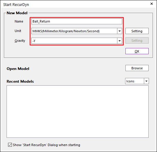
2. Enter the name of the new model as Ball_Return.

3. Set Unit to MMKS.

4. Set Gravity to -Y.

5. Click OK.

1.4.3. Importing Geometry

You will import solid geometry to define the ball channel and container in this model. You will define contact surfaces using the imported geometry.

1.4.3.1. Task Objective

Learn to:

• Import solid geometry in Parasolid format.

• Create a contact surface from the imported geometry using the Face Surface tool.

1.4.3.2. Estimated Time to Complete

5 minutes

1.4.3.3. Importing the CAD Geometry

Now you will import the CAD geometry for the piping system and the container. In this case, the geometry was modeled in the CAD system in the correct locations. You do not need to adjust the geometry position.

1.4.3.3.1. To import the ball return system geometry:

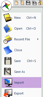
1. From the File menu, click the Import function.

   

2. Set Files of type to ParaSolid File (*.x_t,*.x_b …).

3. In the Basic Tutorials folder of the RecurDyn installation, select the file: Return.x_t.

   (The file path: <InstallDir>\Help\Tutorial\Professional\BallReturn)

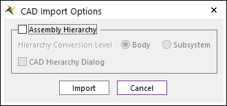
4. Click Open. The CAD Import Options window appears. Clear the Assembly Hierarchy checkbox and click Import.

   

5. Click Import. The Output window appears and displays a message indicating the success of the import.

   Tip

   You can toggle Message window by clicking the Message function from Window group in the Home tab.

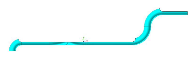
Return Pipe is shown in working window and ImportedBody1 is listed in the Database Window.

Tip

Changing Model View

• You can automatically fit the model view to Working Window using View Control Toolbar.

  • Clicking the Fit tool in View Control Toolbar will fit the model view to Working Window. (Keyboard shortcut for this function is F key.)

  • Clicking the View Snap tool in View Control Toolbar will change the model view to Plane view or Isometric view according to current perspective. (Keyboard shortcut for this function is G key.)

• You can change the graphic rendering mode by changing Rendering Mode in Render Toolbar.

  

  • Wireframe: You can see entities as wire frame.

  • Shade: You can see entities as shade.

  • Shade with Wire: You can see entities as shade with wire.

  • Each Render: You can see entities as specified rendering mode of each entity.

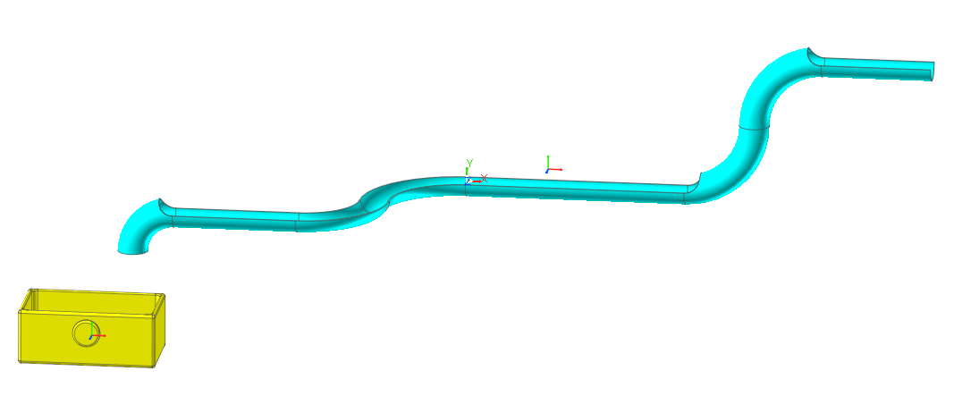
1.4.3.3.2. To import the Container geometry:

Follow the instructions above, but this time, select the file, Container.x_t.

(The file path: <InstallDir>\Help\Tutorial\Professional\BallReturn)

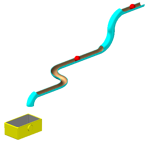
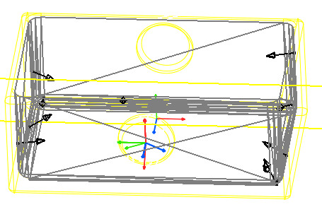
The geometry representing the container appears in the working window (see the figure below) and the body name ImportBody2 appears in the Database window.

1.4.3.3.3. To set the names of both bodies:

1. Display the Properties dialog box for ImportBody1.

2. Select the General page and Change Name to ReturnPipe.

3. Click OK to exit the Properties dialog box.

4. Display the Properties dialog box for ImportBody2.

5. Select the General page and Change Name to Container.

6. Click OK to exit the Properties dialog box.

1.4.3.4. Creating the Ellipsoid Geometry

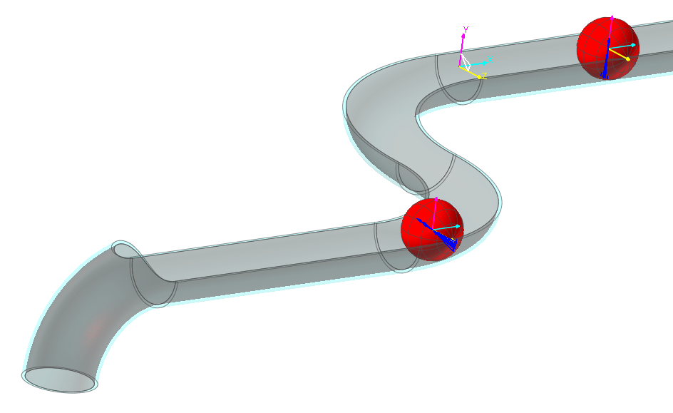
You will create the two bowling balls that are included in this simulation. This process is not only the creation of the ball geometry, but also the setup of the correct mass properties, initial conditions, and names. Ball_1 will be given an initial velocity of 2 m/sec to the left, which provides the energy the initiates the action in the simulation.

1.4.3.4.1. To create the ball geometry:

1. From the Body group in the Professional tab, click the Ellipsoid function. Enter the following:

   • Point: 3000, 1000, 0

   • Distance: 90

2. From the Body group in the Professional tab, click the Ellipsoid function. Enter the following:

   • Point: 700, 0, 0

   • Distance: 90

1.4.3.4.2. To update the ball bodies:

1. Display the Properties dialog box for Body1, the first ball you created:

   • In the General page, change Name to Ball_1.

   • In the Graphic Property page, change Color to Red.

   • In the Body page, change the values using information below.

     • Change Material Input Type to User Input.

     • Change Mass to 30.

     • Change Mass Moment of Inertia (Ixx, Iyy, Izz) to 100000.

     

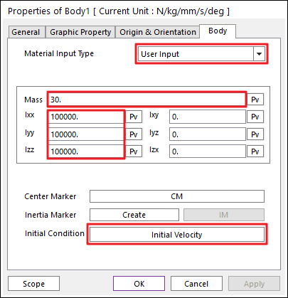
   • Click Initial Velocity. And change the values using information below.

     • In the window that appears, select X Translational Velocity and set the value of the velocity to -2000.

     

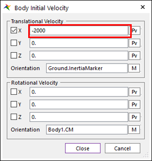
     • Click Close to exit the Body Initial Velocity dialog box.

   • Click OK to exit the Properties dialog box.

2. Display the Properties dialog box for Body2:

   • In the General page, change Name to Ball_2

   • In the Graphic Property page, change Color to Red.

   • In the Body page, change the values using information below.

     • Change Material Input Type to User Input.

     • Change Mass to 30.

     • Change Mass Moment of Inertia (Ixx, Iyy, Izz) to 100000.

   • Click OK to exit the Ball_2 Properties dialog box.

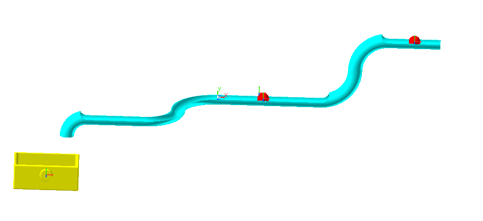
Your model appears as shown in the figure below.

1.4.3.5. Saving the model

From the File menu, click Save.

1.4.4. Defining Joints and Forces

In this chapter, you will create all the necessary joints and forces.

1.4.4.1. Task Objective

You will create:

• A fixed joint to hold the ball return geometry in place.

• A revolute joint to define the pivot point of the container.

• A rotational spring to define the coil spring that controls the rotation of the container as the balls drop into it.

1.4.4.2. Estimated Time to Complete

10 minutes

1.4.4.3. Attaching the Return Pipe to Ground

1.4.4.3.1. To attach the Return pipe to ground using a fixed joint:

1. Click the Fixed Joint function, from the Joint group in the Professional tab.

2. Set the Creation Method to Body, Body, Point.

3. To select Ground as Base Body, click anywhere in the Working Window where there is no geometry. (Or you can enter Ground in the Input Window Toolbar)

4. Click the ReturnPipe geometry as Action Body.

5. Enter 1600, 0, 0 as Point in the Command Toolbar.

1.4.4.3.2. To attach Container to ground using a Revolute Joint:

1. From the Joint group in the Professional tab, click the Revolute Joint function.

2. Set the Creation Method to Body, Body, Point, Direction.

3. To select Ground as Base Body, click anywhere in the Working Window where there is no geometry.

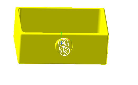
4. Click the Container geometry as Action Body. You will zoom to the Container and define Point and Direction using geometrical information.

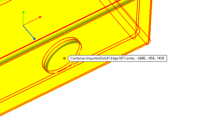
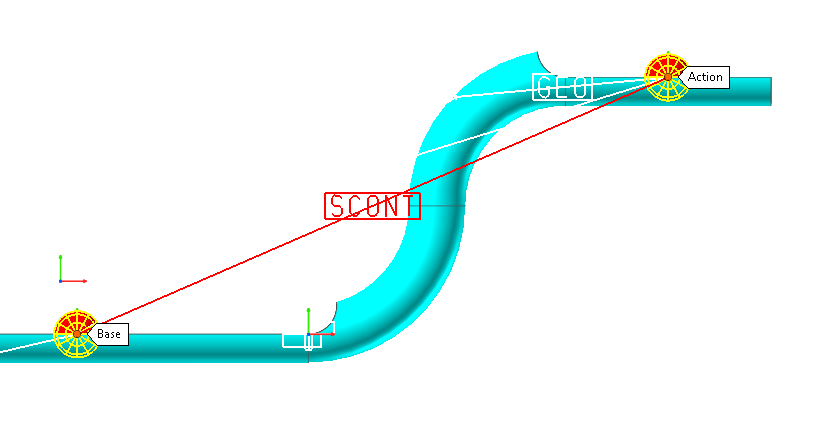
5. Move the cursor over to the inner circle of the fillet on the end of the post as shown at below. When the Tooltip indicating Point value is (-2600, -850, 1430), click the left mouse button to input Point.

   

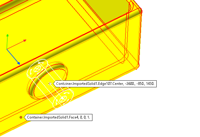
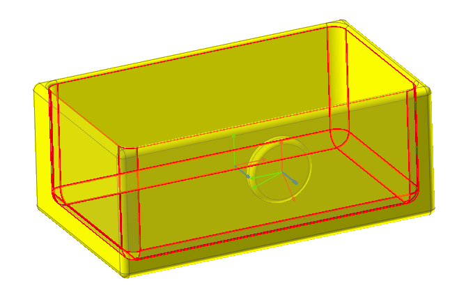
6. Move the cursor over to the square Face of the box as shown in below. When the Tooltip indicating, Normal Vector is (0,0,1), click the left mouse button to input Direction.

   

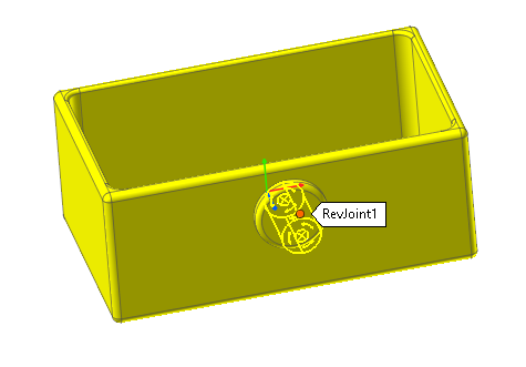
RevJoint1 is created as shown below.

1.4.4.4. Defining the Rotational Spring

You will create a rotational spring that will control the rotation of the container.

1.4.4.4.1. To create the rotational spring:

1. From the Force group in the Professional tab, click the Rotational Spring Force function.

2. Set the Creation Method to Joint.

3. Click the icon of RevJoint1 that you just created.

   

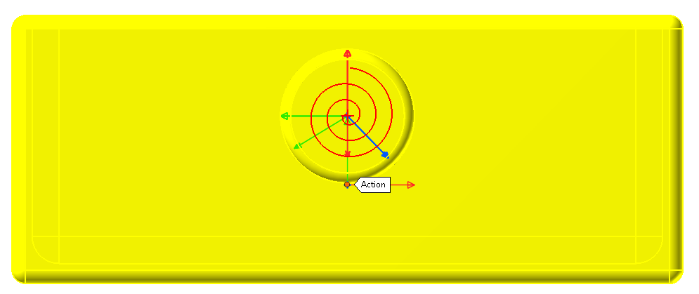
RotationalSpring1 is created as shown below.

1.4.5. Defining 3D Contact

In this chapter, you will create all the contacts between the balls, the balls and ReturnPipe, and the balls and the Container.

1.4.5.1. Task Objective

You will create contact definitions between:

• Ball_1 and the ReturnPipe

• Ball_2 and the ReturnPipe

• Ball_1 and the Container

• Ball_2 and the Container

• Ball_1 and Ball_2

1.4.5.2. Estimated Time to Complete

10 minutes

1.4.5.3. Defining Contact between Ball and the ReturnPipe

You will define FaceSurface in solid geometry of ReturnPipe which is needed to create Contact. And you will define contact between two Balls by using that FaceSurface.

1.4.5.3.1. To create the Contact Surface on the Return geometry:

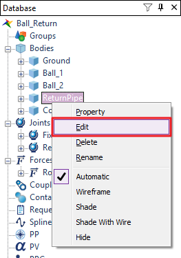
1. Change to Body Edit Mode of the ReturnPipe body:

   • In the Database window, right-click ReturnPipe.

   • From the menu that appears, click Edit.

   

   The Return piping system is now the only geometry in the working window.

2. From the Surface group in the Geometry tab, click the Face Surface function.

3. Set the Creation Method to Solid(Sheet), MultiFace.

4. Click ImportedSolid1 as Solid. The FaceSurf Operation dialog box appears.

5. Click Add/Remove (Continuous) option.

   

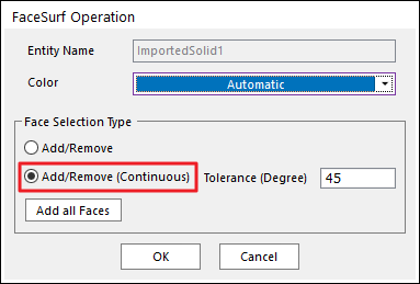
6. Click inner faces of Pipe as shown below.

   

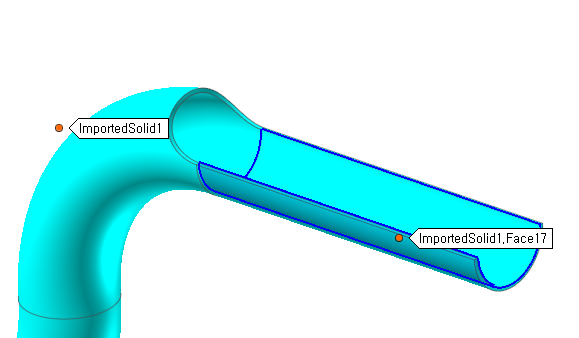
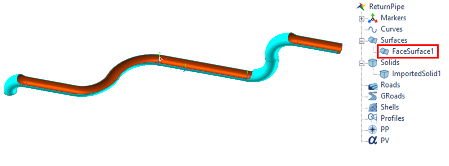
7. When all the inner faces are selected, click OK in FaceSurf Operation dialog box. The newly defined contact surface appears as an item in the Database window under the Surfaces category, FaceSurface1 as shown below.

   

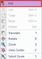
8. Exit the body-editing mode for the Return body by right-clicking the working window, then clicking Exit.

   

1.4.5.3.2. To create the contact between Ball1 and the ReturnPipe

1. Click the Geo Sphere Contact function from Contact group in Professional tab.

2. Set creation method to Surface(PatchSet), MultiSphere.

3. Select ReturnPipe.FaceSurface1 as Surface(PatchSet).

4. Select Ball_1.Ellipsoid and Ball_2.Ellipsoid1 as MultiSphere in this order.

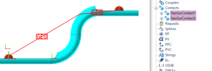
5. Right-Click in Working Window and click Finish Operation. GeoSurContact1 and GeoSurContact2 is created in Database as shown below.

   

1.4.5.4. Defining Contact between Ball and the Container.

Same as ReturnPipe, you will define FaceSurface in Container which is needed to create Contact. And you will define contact between two Balls by using that FaceSurface.

1.4.5.4.1. To create contact surface in Container

1. Change to Body Edit Mode of the Container body:

   • In the Database window, right-click Container.

   • From the menu that appears, click Edit.

2. Click the Face Surface function from Surface group in the Geometry tab.

3. Set creation method to Soild(Sheet), MultiFace.

4. Click ImportedSolid1 as Solid.

5. Select Add/Remove option.

6. In Select Toolbar, change Select State to Add.

   

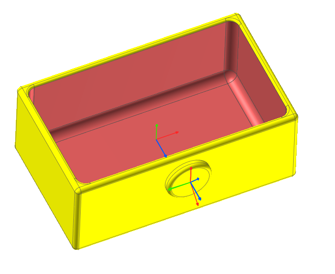
7. Add by clicking inner faces of Container as shown at below. (If you clicked the wrong faces, change Select State to Remove and click the wrong faces.)

   

8. When all the inner faces are selected, click OK in the dialog box. FaceSurface1 is created as shown below.

   

9. Exit the body-editing mode for the Return body by right-clicking the working window, then clicking Exit.

1.4.5.4.2. To create Contact between Ball and Container

1. Click the Geo Sphere Contact function from the Contact group in the Professional tab.

2. Set Creation Method to Surface(PatchSet), MultiSphere.

3. Select Container.FaceSurface1 as Surface(PatchSet).

4. Select Ball_1.Ellipsoid1 and Ball_2.Ellipsoid1 as MultiSphere in this order.

5. Right-Click in Working Window and click Finish Operation. GeoSurContact3 and GeoSurContact4 is created in Database as shown below.

   

1.4.5.5. Defining Contact between Ball_1 and Ball_2

1.4.5.5.1. To create the contact between the balls:

• Click the Sphere to Sphere Contact function from the Contact group in the Professional tab and click the following:

  • Sphere: Ball_1.Ellipsoid1

  • Sphere: Ball_2.Ellipsoid1

  

1.4.5.6. Adjust Contact Surface Resolution of Return

You will adjust the Faceting Resolution of contact surface of Geo Sphere Contact for more accurate simulation results.

1.4.5.6.1. To adjust Faceting Resolution of GeoSurContact1:

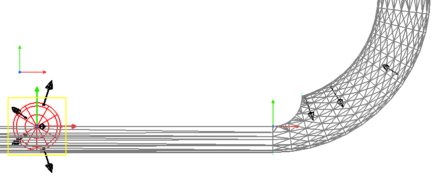
1. Change Rendering Mode to Wireframe in Render Toolbar to see the faceting status of contact surface more clearly.

2. Open Properties dialog of GeoSurContact1. Faceting status of ReturnPipe.FaceSurface1 is shown as figure below.

   

3. Click Contact Geometry at Base Geometry in Geo Contact page. Surface Patch dialog is shown.

   

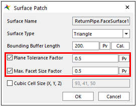
4. Change Plane Tolerance Factor to 0.5.

5. Check the Max. Facet Size Factor option and change it to 0.5.

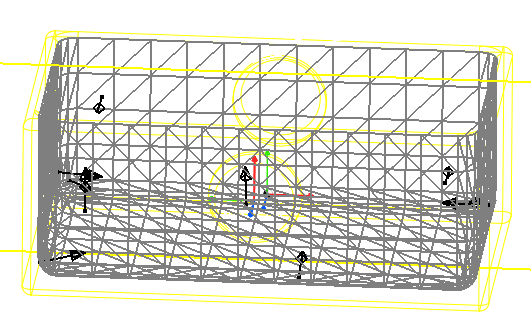
6. Click OK in Surface Patch dialog. You can see that facet size has become more detailed as shown below.

   

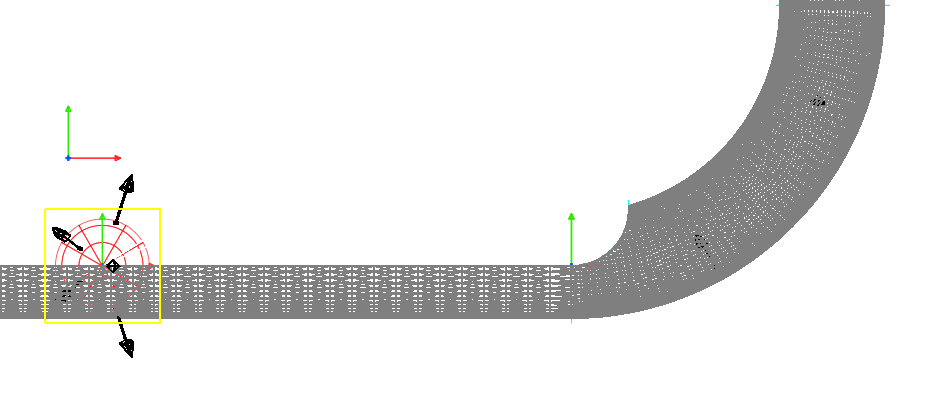
7. Click OK in GeoSurContact1 dialog. You do not need to change contact surface of GeoSurContact2 because it is defined as same geometry of GeoSurContact1.

1.4.5.6.2. To adjust Faceting Resolution of GeoSurContact3:

1. Open the Properties dialog of GeoSurContact3. Faceting status of Container.FaceSurface1 is shown as figure below.

   

2. Click Contact Geometry at Base Geometry in Geo Contact page. Surface Patch dialog is shown.

3. Check the Max. Facet Size Factor option and change it to 1.

4. Click OK in Surface Patch dialog. You can see that facet size has become more detailed as shown below.

   

5. Click OK in GeoSurContact3 dialog. You do not need to change contact surface of GeoSurContact4 because it is defined as same geometry of GeoSurContact3.

6. Change Rendering Mode to Shade With Wire in Render Toolbar.

1.4.5.6.3. To modify the property of GeoSurContact

You will modify the value about the contact property between ReturnPipe and Ball.

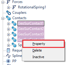
1. From GeoSurContact1 to GeoSurContact4, select 4 Contacts from Database. Then right-click holding Ctrl key to click Properties.

   

   Multi-Properties dialog is shown which can change the properties of selected entities.

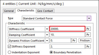
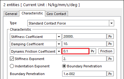
2. In Characteristic page, change the values using information below.

   • Stiffness Coefficient: 20000

     

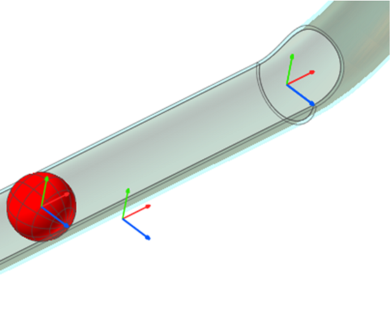
   You will set the options about Force Display to visually check the contact force of ReturnPipe and Two Ball in animation.

3. In Geo Contact page, change the values using information below.

   • No. of Max Contact Points: 20

   • Force Display: Action

     

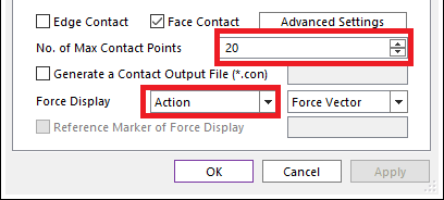
4. Click OK.

1.4.5.6.4. To modify the graphic property of ReturnPipe

You will adjust graphic transparency of ReturnPipe to visually check the contact force of ReturnPipe and Ball_2 in animation.

1. Open Properties dialog of ReturnPipe.

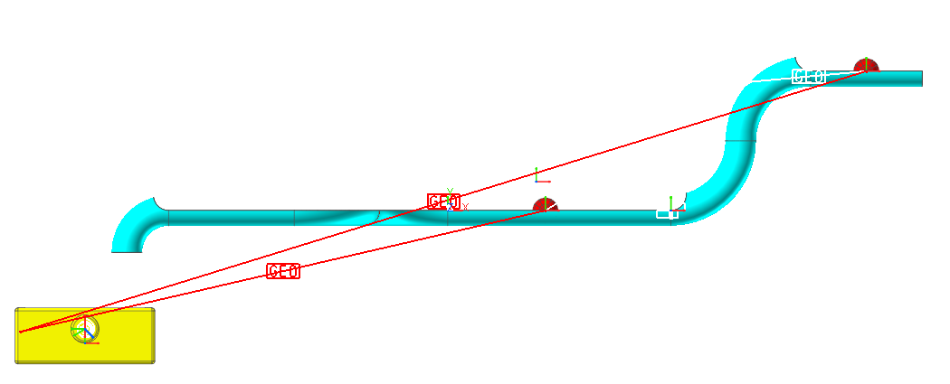
2. In Graphic Property page, check Apply Transparency for All Graphics belong to Body and move Transparent Level slider to right as shown below.

3. Click OK.

   

1.4.5.6.5. To hide the icon

1. In Render Toolbar, click the Icon Control tool.

2. Uncheck All Icons to disappear the icons on Working Window.

   

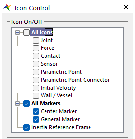
3. Close Icon Control window

1.4.5.7. Saving the Model

Take a moment to save your model before you continue with the next chapter.

1.4.6. Analyzing and Reviewing the Model

In this chapter, you will run a simulation of the model you just created. You will examine the results and think about what to change to make sure the results are correct.

1.4.6.1. Task Objective

Learn to use the more advanced aspects of plotting, including playing animations with the plots and using the Plot Template and Trace Data tool.

1.4.6.2. Estimated Time to Complete

5 minutes

1.4.6.3. Performing Dynamic/Kinematic Analysis

In this section, you will run a dynamic/kinematic analysis to view the effect of forces and motion on the model you have just created.

1.4.6.3.1. To change options about Simulation Output.

To use Output File Name function efficiently, the Create Output Folder option is turned off.

1. From the Model Settings group in the Home tab, click the Simulation Setting function. The Simulation dialog box will appear.

2. Select the General page. Make sure the Create Output Folder check box is not checked.

   

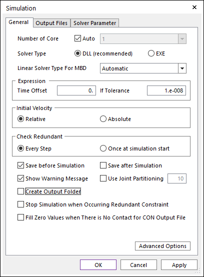
3. Click OK

1.4.6.3.2. To perform a Dynamic/Kinematic analysis:

1. Click the Dynamic / Kinematic Analysis function from the Simulation Type group in the Analysis tab. The Dynamic/Kinematic Analysis dialog box appears.

2. Define the End Time of the simulation and the number of Steps:

   • End Time: 4

   • Step: 200

   • Plot Multiplier Step Factor: 10

     

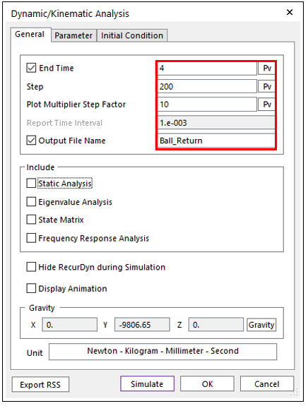
3. Select Output File Name, and then enter the output file name: Ball_Return.

4. Click Simulate.

1.4.6.4. Examine the result

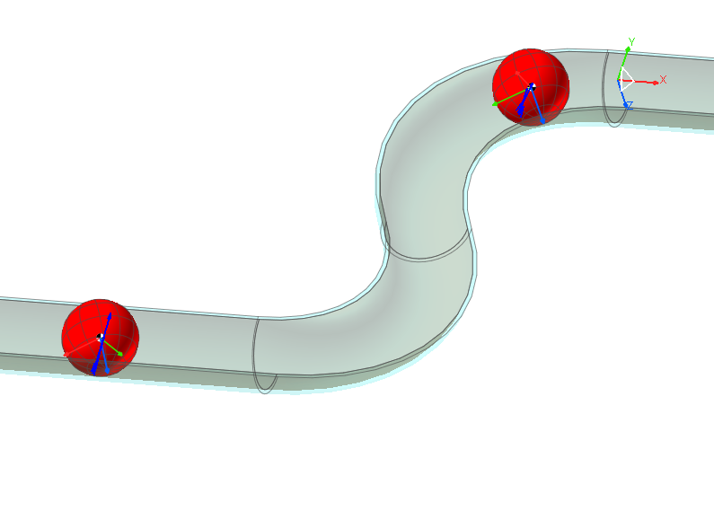
1.4.6.4.1. To examine the animation result

• Click the Play function from the Animation Control group in the Analysis tab to play animation.

  Ball_1 (in the right) moves to the left and affects Ball_2. Ball_2 moves along the path in ReturnPipe and fall into the Container.

  

  Overall behavior seems appropriate. However, if you move the Animation step by step and observe Ball_2, it doesn’t roll because ReturnPipe and Ball_2 don’t have friction force between them.

1.4.6.4.2. To examine the Plot result

1. Click the Plot Result function from the Plot group in the Analysis tab. Working window changes to Plot Window.

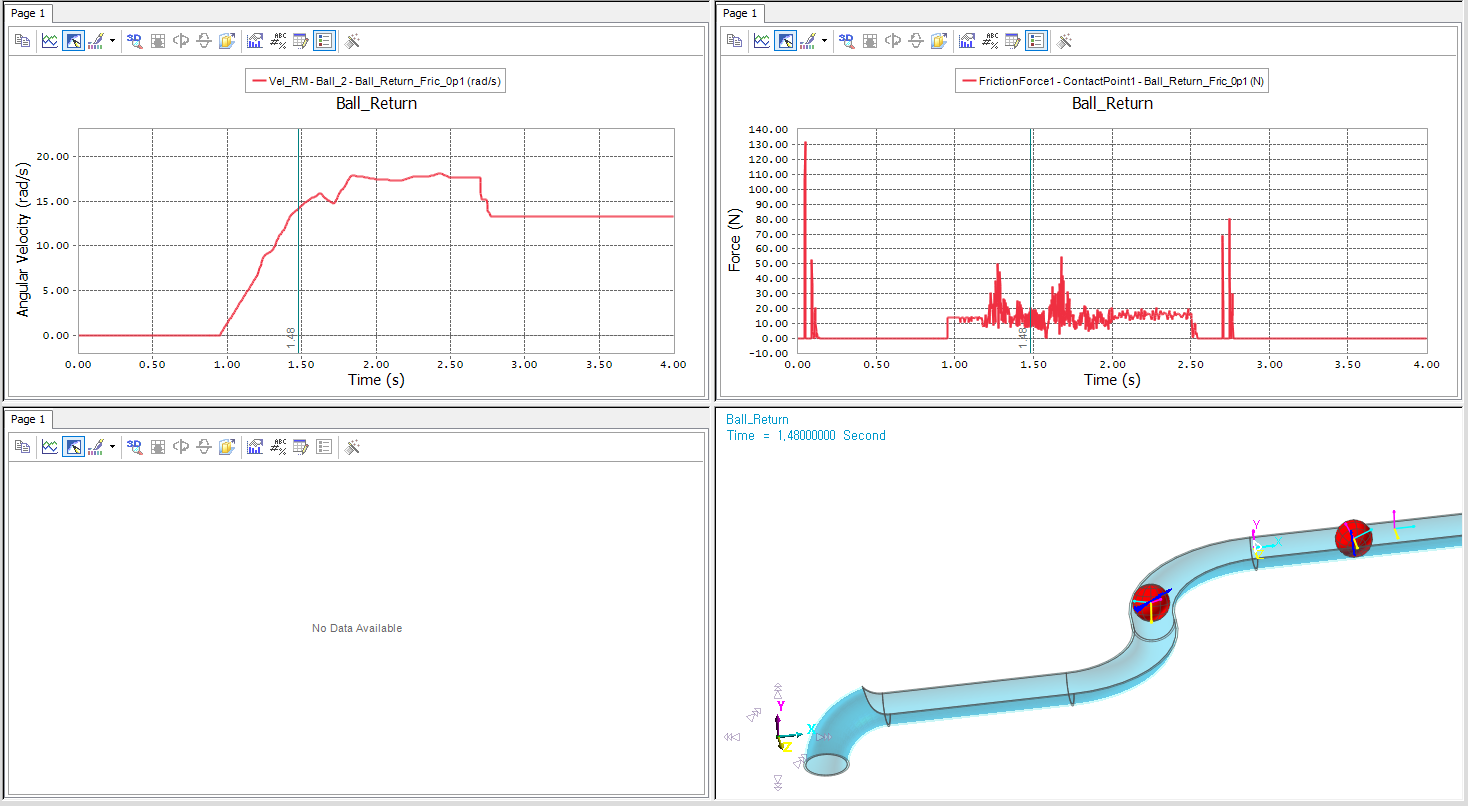
2. Click the Show All Windows function from the Windows group in the Home tab to display four plotting windows.

3. Click the Upper left window to make that pane active and double click Vel_RM in the Database following path below.

   • Ball_Return -> Bodies -> Ball_2 -> Vel_RM

4. Click the upper right window to make that pane active and double click FrictionForce1 in the Database following path below.

   • Ball_Return -> Contact -> Geo Contact -> GeoSurContact2 -> ContactPoints -> ContactPoint1 -> FrictionForce1

5. Click the lower right window to make that pane active and click LoadAni from Animation group in the Tool tab.

6. Click Yes when the warning message appears.

7. Click the Play function and check the animation.

   

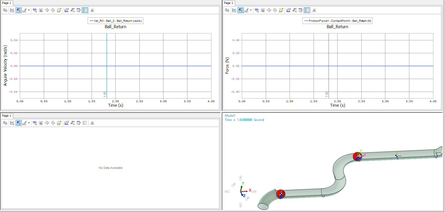
As we already checked, Ball_2 does not roll because ReturnPipe and Ball_2 do not have friction force between them. For more realistic results, you will modify the friction information in the Contact between ReturnPipe and Ball_2.

1.4.6.4.3. To create Plot Template

You will create Plot Template to reduce the inconvenience of redrawing plot results after each simulation.

1. Click the Export Plot Template function from the Export group in the Home tab. The Export Plot Template Settings dialog is shown. The dialog shows the list of properties of drawn plots.

2. Exclude below items from the list.

   • UpperLeft > Page1 > Chart > Axes > Axis Y > Scale

   • UpperRight > Page1 > Chart > Axes > Axis Y > Scale

   (If you do not exclude Scale of Axis Y, it will not automatically scale when drawing the next plot.)

   

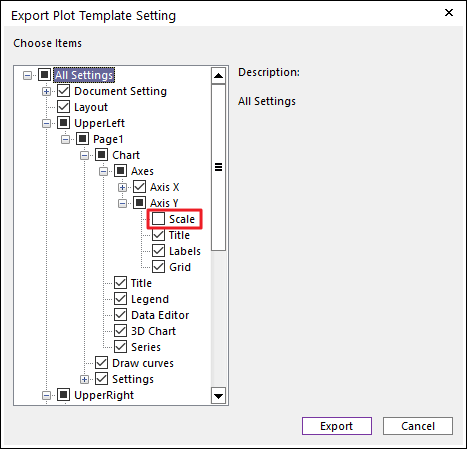
3. Click Export to save Template file.

1.4.6.5. Running a New Simulation

1.4.6.5.1. To define the friction value for the contact between Ball and ReturnPipe

1. Select GeoSurContact1 and GeoSurContact2 from Database. Then right-click holding Ctrl key to click Properties.

   

   Multi-Properties dialog is shown which can change the properties of selected entities.

2. In Characteristic page, change the values using information below.

   • Dynamic Friction Coefficient: 0.1

     

3. Click OK.

1.4.6.5.2. Connect Plot Template file before running a new simulation

1. Click the Plot Template Setting function from the Plot group in the Analysis tab.

2. Check Use the Default Template File(*.template) when the Template dialog is shown.

3. Select Use the Specified File and enter the file path where you saved the *.template file.

   

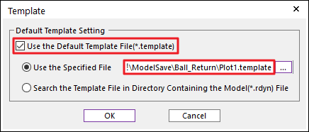
4. Click OK.

1.4.6.5.3. To perform a dynamic/kinematic analysis:

1. Click the Dynamic / Kinematic Analysis function from the Simulation Type in the Analysis tab. The Dynamic/Kinematic Analysis dialog box appears.

2. Change the file name: Ball_Return_Fric_0p1

   

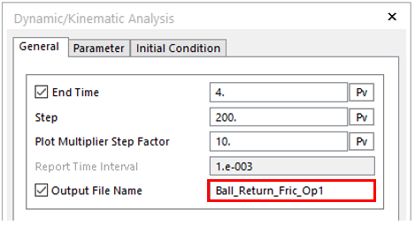
3. Click Simulate.

1.4.6.5.4. To examine the animation result

• Click the Play function from the Animation Control group in the Analysis tab.

  If you move the Animation step by step and observe Ball_2, it rolls because ReturnPipe and Ball_2 now have friction force between them.

  

1.4.6.6. Comparing the Results of the Two Simulations

1.4.6.6.1. To compare the result from previous analysis using Plot Add

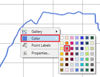
1. Click the Plot Add function from the Plot group in the Analysis tab.

   Previous Plot Window opens again and plot from new simulation result is automatically drawn. You will change the color of graph to separate the overlapped two graphs.

2. In the Plot Window, select the newly drawn graph and right-click it.

3. Change the Color to Red when the Pop-up menu appears.

   

If you compare the two plot results, you can check that Contact Friction Force is generated between Ball_2 and ReturnPipe. Also, you can check that Angular Speed is generated from Contact Friction Force.

1.4.6.6.2. To draw the graph simultaneously using Multi Draw

1. Click the lower left window.

2. Unfold to see Vel_TM in the Database following path below.

   • Ball_Return -> Bodies -> Ball_2 Vel_TM

3. Right-click it and click Multi Draw in the pop-up menu.

   

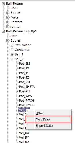
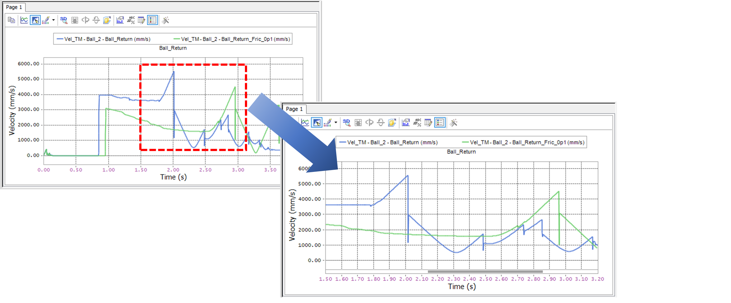
   Graph about Ball_Return and Ball_Return_Fric_0p1 are simultaneously drawn.

   

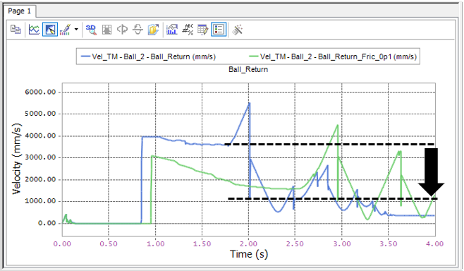
   If you compare the two results, you can see that the velocity of Ball_2 has decreased when it moves in the ReturnPipe because of friction force.

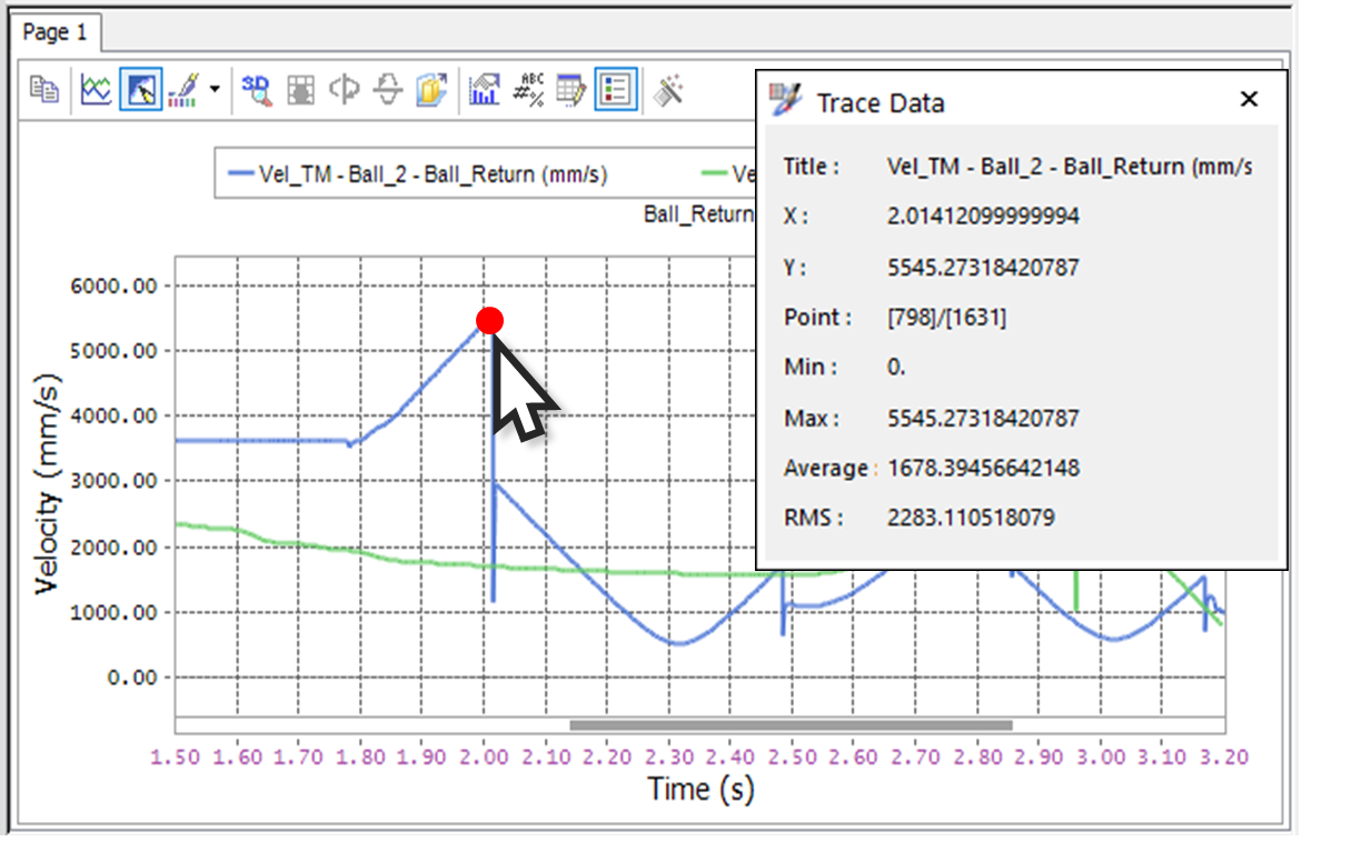
1.4.6.6.3. To find the peak value using Trace Data:

1. Click the Select Zoom function from the View group in the Home tab.

2. In the Plot Window where the Vel_TM graph is, drag the area where the peak value is located as shown below. You can see the area you dragged magnified as shown below. The highest value of Vel_TM graph is where the Ball_2 free-falls.

   

3. From the Tools group in the Home tab, click the Trace Data function.

4. Place the cursor at the peak value of the graph. Data Display appears as shown below.

   • The first row contains the animation frame number.

   • The second row contains the X value (time).

   • The third row contains the Y value (velocity).