8.4. RFlex Crankshaft Tutorial (Durability)

8.4.1. Introduction

Fatigue and durability analyses are designed to determine how long a flexible body or specific area of a flexible body modeled in RecurDyn can stably endure various dynamic loads. Such analyses can also determine how stable a body is. The focus on time distinguishes these forms of analysis from other analysis methods, such as those used to determine maximum stress and maximum deformation rates.

RecurDyn, in consideration of the flexibility of the model, supports RFlex of FFlex bodies in multi-body dynamic models. Therefore, this tutorial teaches you how to use the RecurDyn/Durability module to analyze the durability of both the FFlex bodies and the RFlex bodies.

The model being used in this tutorial is a simplified 4-cylinder internal combustion engine. The crankshaft in this model has been replaced with an RFlex body, and the combustive explosion process occurring in the four cylinders push the pistons to provide a dynamic load. The durability analysis in this tutorial determines the stability and durability of the crankshaft design.

8.4.1.1. Task Objectives

This tutorial covers the following:

• Replacing a flexible body using RecurDyn/RFLEX

• Verifying stresses using RecurDyn/RFLEX

• Recognizing the requirements for the durability analysis

• Obtaining durability analysis results

• Analyzing durability analysis results

8.4.1.2. Requirements

This tutorial is intended for intermediate users who have read and understood the basic tutorial as well as the FFlex and RFlex tutorials available from RecurDyn. If you have not completed these tutorials, then you are advised to complete them before proceeding with this tutorial. In addition, this tutorial requires a basic understanding of dynamics and the finite element method.

8.4.1.3. Procedures

This tutorial is composed of the following procedures. This table also shows the time required to complete each task.

Procedures	Time (minutes)
Calling an Rdyn model‏	10
Replacing an RFlex body.	15
Creating a patch set to verify the fatigue results	5
Conducting a fatigue evaluation	25
Verifying the fatigue results	10
Total	65

8.4.1.4. Estimated Time to Complete

65 minutes

8.4.2. Calling the Initial Model

8.4.2.1. Task Objective

This chapter teaches you how to open the initial model, simulate it, and observe how a 4-cylinder engine model operates.

8.4.2.2. Estimated Time to Complete

10 minutes

8.4.2.3. Calling the Rdyn model

8.4.2.3.1. To run RecurDyn and call the initial model:

1. On the Desktop, double-click the RecurDyn icon. When the Start RecurDyn dialog window appears, close it.

2. From the File menu, click Open.

3. Under the Durability tutorial path, select the RD_Durability_4Cyl_Engine_Start.rdyn file.

   (The file path: <InstallDir>\Help\Tutorial\PostAnalysis\Durability\RFlexCrankshaft)

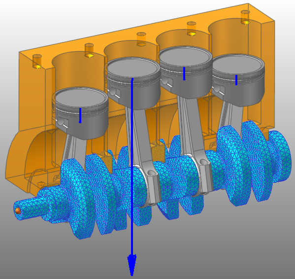
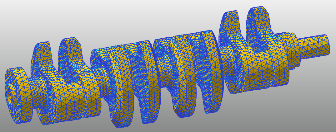
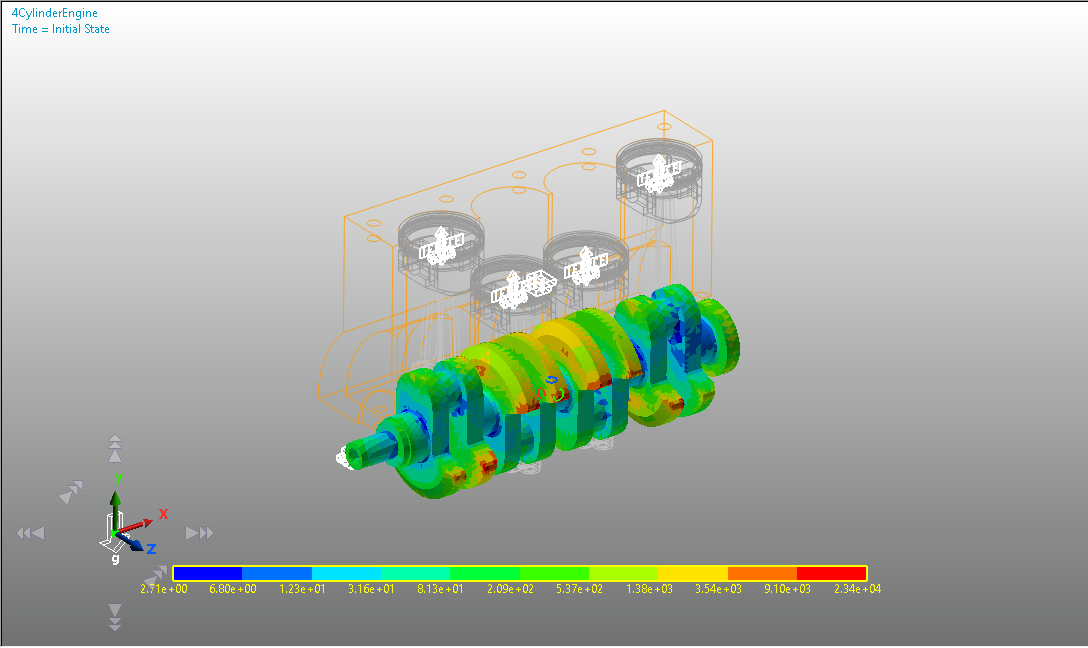
4. Click Open. The model is shown below opens.

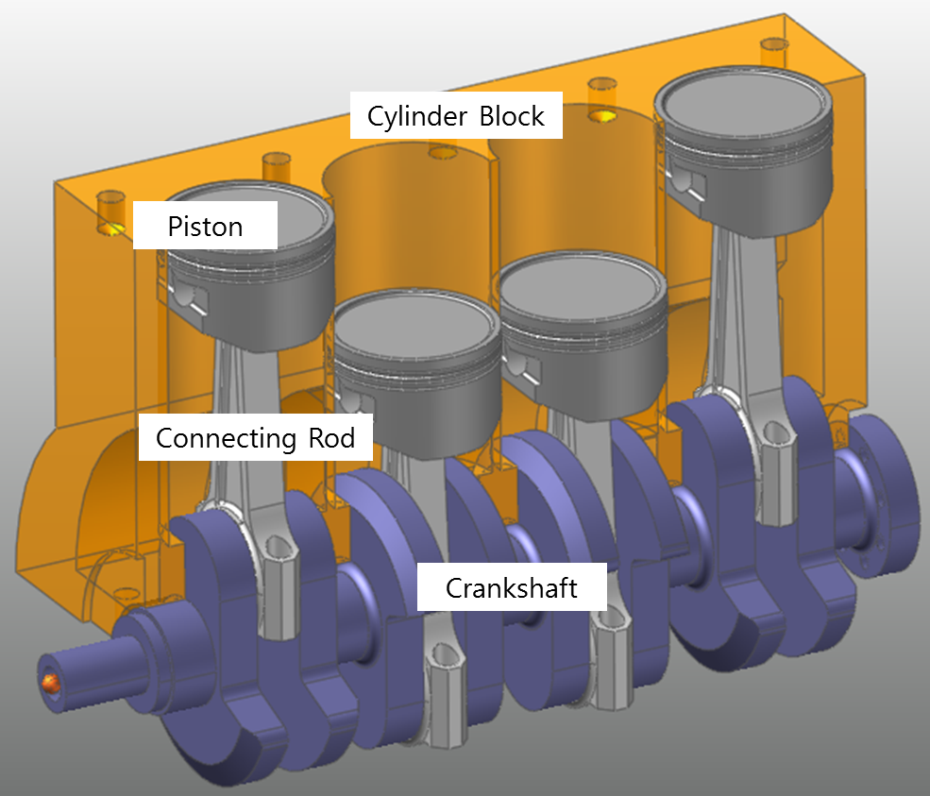
The above figure shows a model of an inline 4-cylinder engine, which consists of a cylinder block, pistons, connecting rods, and a crankshaft. In an actual combustion engine, a gas explosion forces the four pistons vertically into the cylinder block, causing the connecting rods on each piston to rotate the crankshaft. In order to simulate such a process in RecurDyn, you must simulate the timing of the gas explosion in the force profile and directly assign it to the piston bodies as a vibration force.

8.4.2.3.2. To save the initial model:

• From the File menu, click Save As.

  (Save this model in the different path because it is impossible to simulate directly in the tutorial path.)

8.4.2.4. Running the Initial Simulation on the 4-Cylinder Engine Model

In this task, you will run an initial simulation on the model to understand how it operates.

8.4.2.4.1. To run the initial simulation:

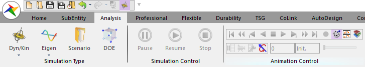
1. From the Simulation Type group in the Analysis tab, click the Dynamic/Kinematic Analysis function.

2. The Dynamic/Kinematic Analysis dialog window appears.

3. Verify the simulation conditions and click Simulate.

8.4.2.4.2. Viewing the results:

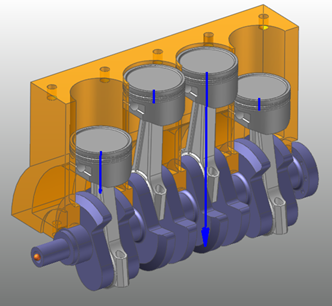
When your click the Play function from the Animation Control group in the Analysis tab, the fuel explodes in all four pistons in the following order:

Piston_1 -> Piston_3 -> Piston_4 -> Piston_2. You can verify the size of the arrows indicating the force in the animation. Generally, four processes occur in each stroke of the piston (intake -> compression -> explosion -> exhaust). However, in the dynamic model used in this tutorial, only the gas explosion force generated by explosion is significant. Thus, the force profile was created with respect to the timing of the explosive force, and it was modeled in order to assign force to each piston in the appropriate order.

8.4.3. Creating an RFlex Body

This chapter teaches you how to conduct a fatigue analysis on Flexible Bodies.

8.4.3.1. Task Objective

This task teaches you how to replace an existing rigid body with a flexible body using the RFlex body feature provided in RecurDyn/RFlex and conduct a fatigue analysis on the flexible body.

8.4.3.2. Estimated Time to Complete

15 minutes

8.4.3.3. Creating an RFlex Body

8.4.3.3.1. To create the RFlex body:

1. From the RFlex group in the Flexible tab, click the Import RFI function.

2. Change the modeling option to Body.

3. In the Working window, select the Crankshaft, as shown below.

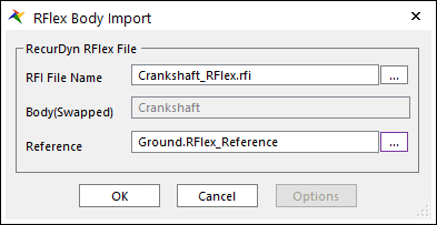
4. The RFlex Body Import dialog window appears.

   

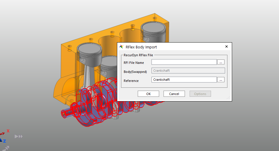
5. In the RFlex Body Import dialog window, perform the following:

   • Click the … button to the right of the RFI File Name text box.

   • Select the Crankshaft_RFlex.rfi file, which is located in the same folder as the RD_Durability_4Cyl_Engine_Start.rdyn file.

   • Click the … button to the right of the Reference text box.

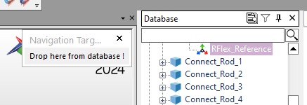
   • In the Database Window, under the Ground group, drag the RFlex_Reference marker and drop it in the Navigation Target Window, as shown in the figure to the below.

     

6. Verify that the most recently selected conditions match those shown in the figure to the below, and then click OK.

   

7. The RFlex body will replace the Crankshaft Body.

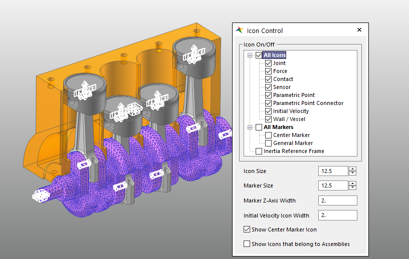
8. Click the Icon Control tool in Render Toolbar, select All Icons and view the results. Ensure that all of the joints that are applied to the existing crankshaft are still applied to the RFlex body. After verifying the joints, clear the selected icons.

   

8.4.3.4. Conducting the Dynamic Analysis on the RFlex Body and Reviewing the Results

8.4.3.4.1. To conduct a dynamic analysis on the RFlex body:

1. Select and right-click Crankshaft and click Properties.

2. The Properties of RFlexBody1 dialog window appears.

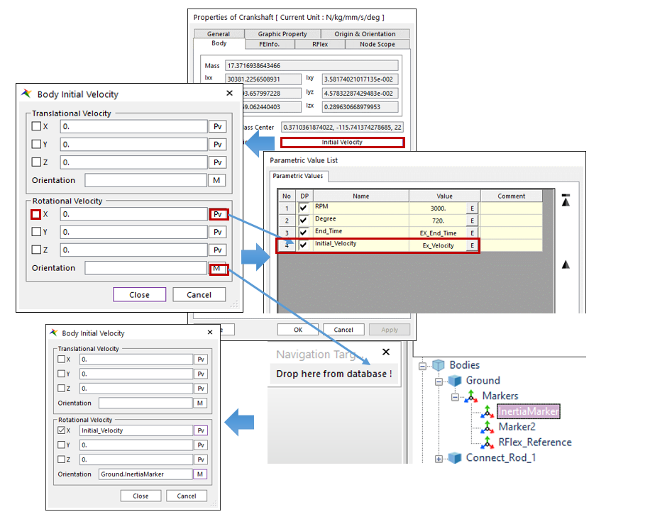
3. In the Properties of RFlexBody1 dialog window, on the Body page, click Initial Velocity.

4. In the Body Initial Velocity dialog window, perform the following:

   • In the Rotational Velocity group, select the X checkbox, and click PV.

   • Select Initial_Velocity in the Parametric Value List dialog window.

   • Click M to the right of the Reference Marker text box.

   • In the Database Window, drag the Ground Inertia Marker and drop it in the Navigation Target window. Click Close to close the dialog window.

5. The entire procedure is shown below.

   

6. From the Simulation Type group in the Analysis tab, click the Dynamic / Kinematic Analysis function. When the dialog window appears, click Simulate to run the analysis without changing the settings.

7. It does not take long to complete the simulation. During the simulation, the animation is similar to the previous crankshaft body animation.

   

8.4.3.4.2. To display the distribution of stress in the RFlex body:

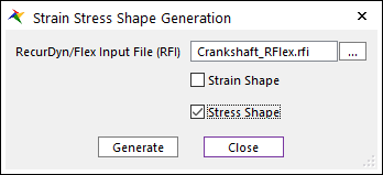
1. From the RFlex group in the Flexible tab, click the Stress Strain Shape Generation function.

2. The Stress Shape Generation dialog window appears.

3. In the Stress Shape Generation dialog window, perform the following:

   • For the RecurDyn/Flex Input File, specify the RFI file.

   • Select Stress Shape.

   • Click Generate.

     

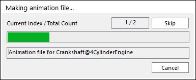
4. The status dialog window appears to display the stress shape creation progress, as shown in the figure on the below.

   

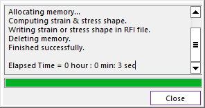
5. After the stress shape is created, click Close in both dialog windows.

   Tip

   Since the RFI file provided in this tutorial includes only the mode shape information, you must add the stress shape information to the existing RFI file in order to view the stress result. Naturally, this process will increase the size of the RFI file.

   To view the simulated stress results in the contour view of RecurDyn/RFlex, you must create output files, *.srd files, in the output folder. These files save the stress results for all the nodes in the RFlex body. You can still see the results if you do not create output files, but it may slow the contour animation.

6. Click the Output Regenerator function from the RFlex group in the Flexible tab.

   The Output File Generator dialog window appears, as shown in the figure to the below.
   

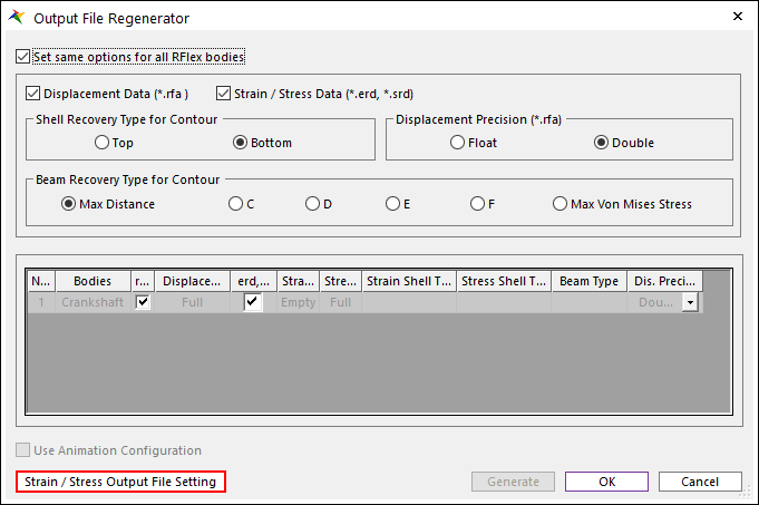
7. Click Output File Setting. The Output File Setting dialog appears as shown in the figure on the below.

   

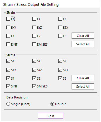
8. In the Stress group, click Select All.

9. Click Close.

   Tip

   When creating an output file, only the Von-Mises, Sx, Sy, and Sz tests are included to reduce the file size. If you would like to view other results in the contour, you must select every check button.

10. In the Output File Generator dialog window, click Generate.

11. When the file is generated, the Stress column in the Information table changes from Empty to Full.

    Tip

    If the output file was created using the default settings, then the Stress column changes to Partial rather than Full. This is because out of 11 stress tests, only Von-Mises, Sx, Sy, and Sz components are conducted.

    

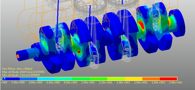
12. In the RFlex group, click the Contour function. The Contour dialog window appears, as shown below.

    

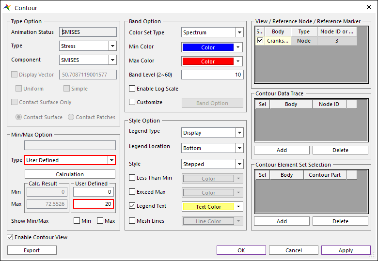
13. In the Contour dialog window, perform the following:

    • In the Min/Max Option group, click Calculation.

    • In the Min/Max Option group, set the Type to User Defined.

    • In the Max text box, type 20.

    • Click OK to close the dialog window.

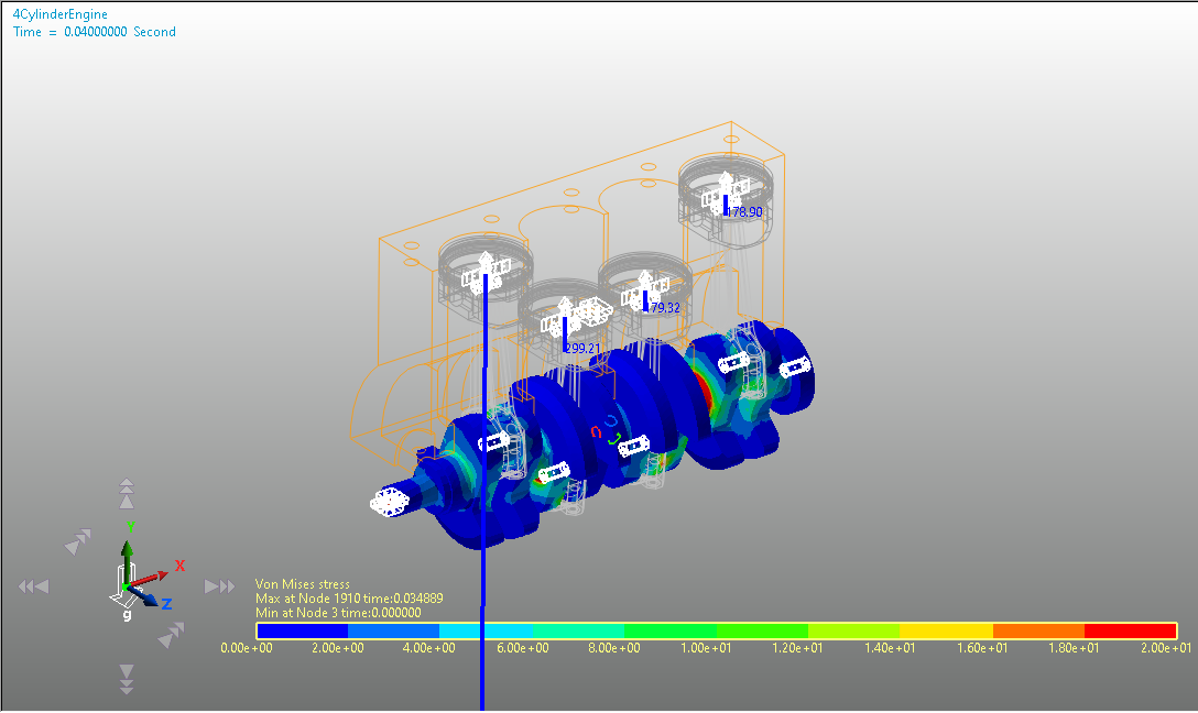
14. Click Animation Play. The results appear on the model, as shown in the below figure.

    

8.4.4. Conducting the Durability Analysis

8.4.4.1. Task Objective

This chapter teaches you how to analyze the durability of the RFlex body.

8.4.4.2. Estimated Time to Complete

30 minutes

8.4.4.3. Conducting the Durability Analysis

8.4.4.3.1. To create a patch set:

1. Double-click Crankshaft to enter RFlex Body Edit Mode.

2. From the Set group in the RFlex Edit tab, click the Patch Set function.

3. Click Add/Remove, as shown below. Then, hold down the left mouse button and drag the cursor across the model to select the entire body.

   

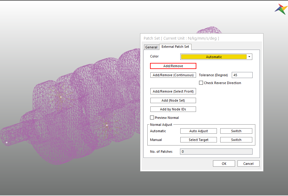
4. Right-click the selected body and click Finish Operation in the context menu.

5. In the Patch Set dialog window, click OK.

6. After the patch set has been created, click the Exit function in the Exit group of the RFlex Edit tab to return to the parent mode.

   

8.4.4.3.2. To retrieve the animation file:

• From the Animation Control group in the Analysis tab, click the Reload the last animation file function, as demonstrated below.

Note that all of the animation-related buttons are activated.

Tip

When creating the patch set for the RFlexBody1, it may appear as though the previous analysis results are no longer available. However, that procedure does not affect the dynamic analysis results. Therefore, there is no need to perform the dynamic analysis again. You can simply retrieve the animation file, or the RAN file, for the previously analyzed result.

8.4.4.3.3. To set the analysis preferences:

1. From the Durability group in the Post Analysis tab, click the Preference function to open the Preference dialog window.

2. In the Preference dialog window, on the Material page, specify the path to the Material Library file for the fatigue analysis.

   (C:\Users\<Your Windows Login ID>\Documents\RecurDyn\<RecurDyn Version> or an equivalent path depending on the OS environment)

3. On the Fatigue Influencing Factors page, in the Fatigue Factors group, set the Notch Factor Amp (Kf, Kt) to 1.2, as shown below.

   

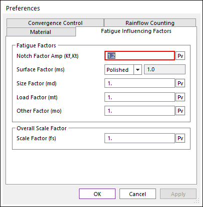
4. The Notch Factor increases the analytically derived stress value to account for stress concentrations due to cracks, holes, and notches (V grooves) caused by the design and processing of the structure. Therefore, the larger the notch factor value is, the more severe the durability analysis will be.

5. In the Preference dialog window, do not change the Convergence Control or Rainflow Counting values, and click OK.

8.4.4.3.4. To conduct the fatigue evaluation:

1. From the Durability group in the Post Analysis group, click the Fatigue Evaluation function.

2. The Fatigue Evaluation dialog window appears.

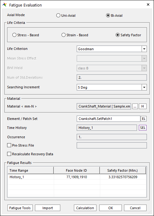
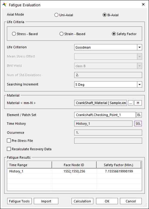
3. In the Fatigue Evaluation dialog window, perform the following:

   • For the Axial Mode, select Bi-Axial.

   • Change the Life Criteria to Safety Factor.

   • For the Life Criterion, select Goodman.

   • Set the Searching Increment to 5 Deg.

     

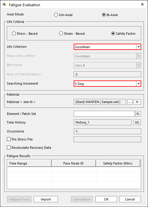
4. In the Materials group, click ….

5. When the Material Manager dialog window appears, perform the following:

6. Select and right-click [Steel] 1020, and click Make Active in the context menu, as shown in the figure to the below.

   

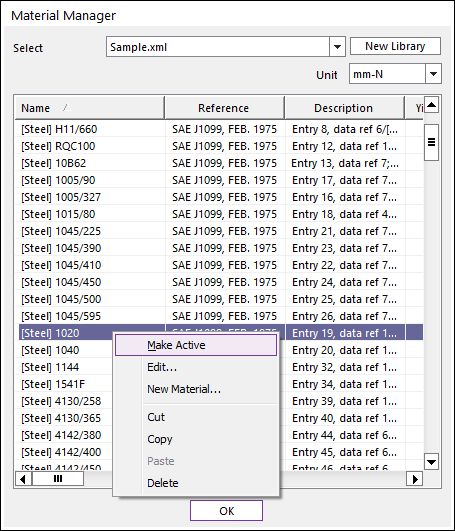
7. Click OK.

8. Click EL to the right of the Element/Patch Set text box.

9. Select the Patch Set for RFlexBody1.

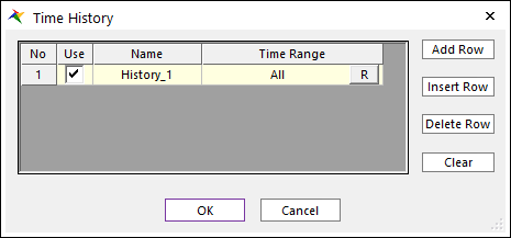
10. A Time History set is defined already, in the Time History dialog window. To change the range of time, click R.

    

11. In the Time Range dialog window, click All.

    

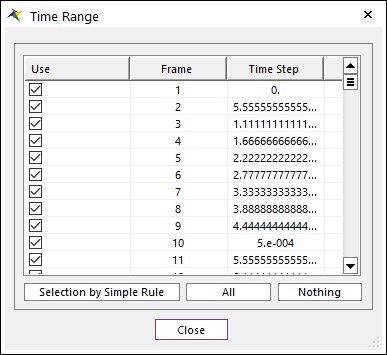
12. Click Close in the Time Range dialog window.

13. Click OK.

14. Click Calculation.

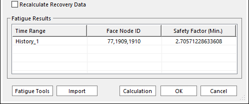
15. A progress bar appears to display the fatigue analysis progress. Upon completion of the analysis, the results will appear in the results group, as shown in the figure to the below.

    

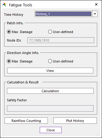
16. In the Fatigue Evaluation dialog window, click Fatigue Tools.

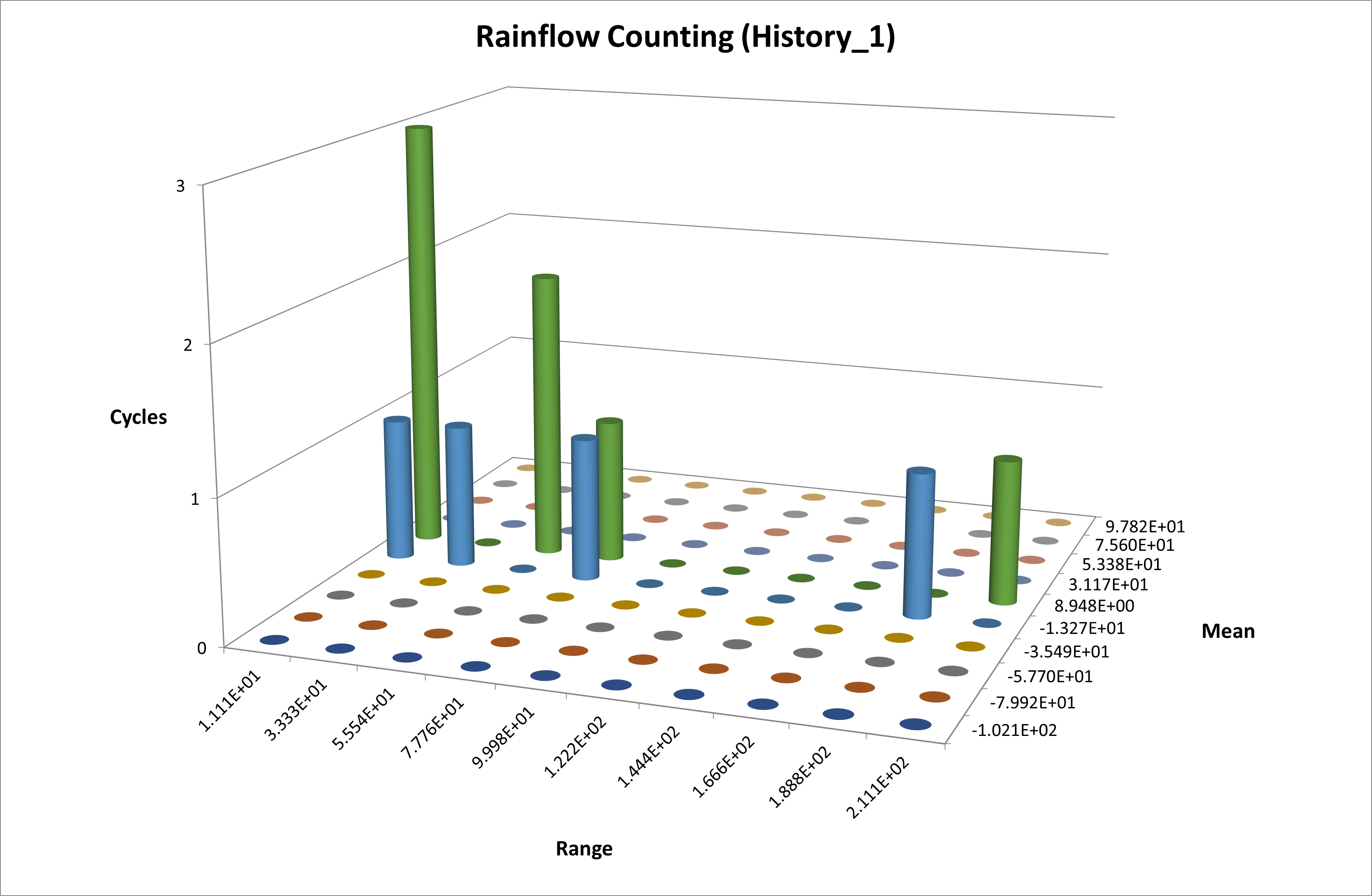
    • Click the Rainflow Counting button in the Fatigue Tools dialog.

      

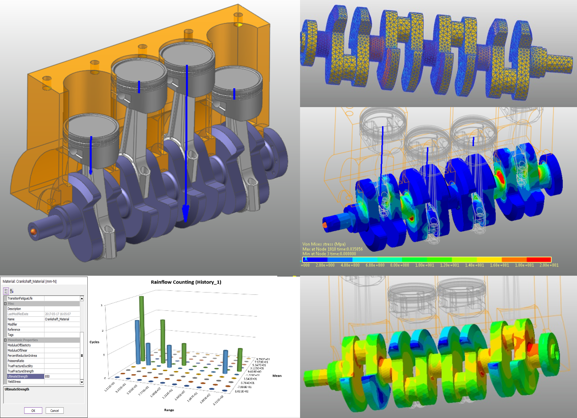
    As shown below, the Rainflow Counting results in the Excel are based on the Stress Time History applied to the patch zone where the damage is largest. The results are displayed in the numbers of cycles according to the stress amplitude and the mean stress.

    

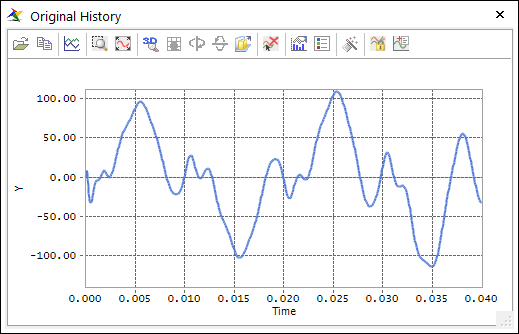
• Click the Plot History in this dialog.

  As shown below, it is possible to check the Stress Time History on the patch which has the maximum damage results among the defined patches.

  

8.4.4.3.5. To verify the contour results:

1. From the Durability group in the Post Analysis group, click the Contour function.

2. The Durability Contour dialog window appears.

3. In the Durability Contour dialog window, perform the following:

   • Click Calculation.

   • Select Enable Log Scale.

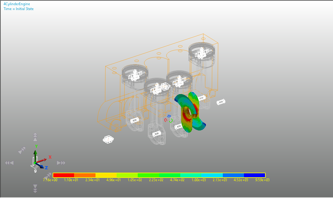
   • Click Contour View to view the results.

     

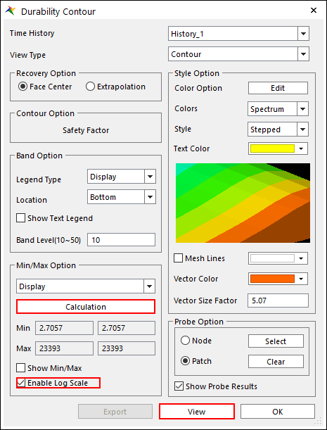
4. To make the results more visible, click Edit in the Style Option group of the Durability Contour dialog window, and change the colors as follows.

   

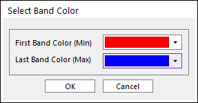
5. Click Contour View again to highlight the least durable sections in red, as shown below. This makes it easier to identify the areas with a relatively short fatigue life.

   Tip

   At this point, if you would like a more detailed Contour Plot, then select Wireframe in the toolbar before viewing the results.

   

8.4.4.3.6. To change the materials and conduct another fatigue evaluation:

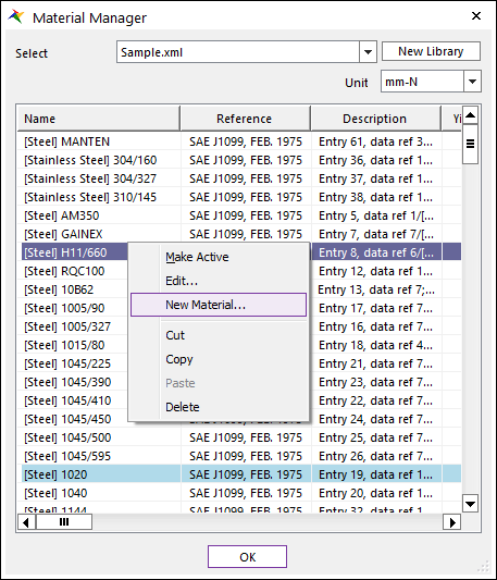
1. In the Fatigue Evaluation dialog window, in the Material group, click …. The Material Manager dialog window appears.

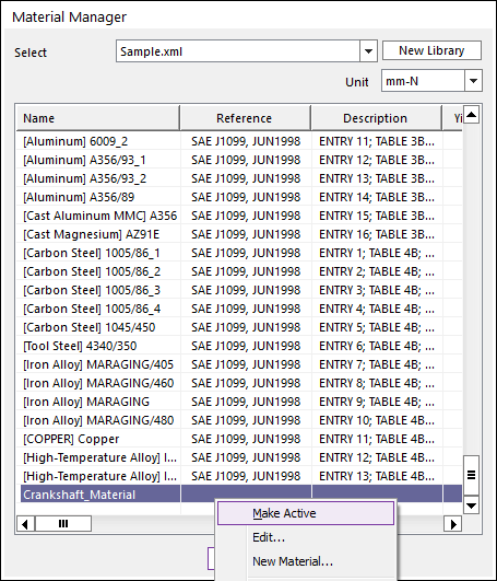
2. Right-click the list, and click New Material in the context menu, as shown in the figure to the below.

   

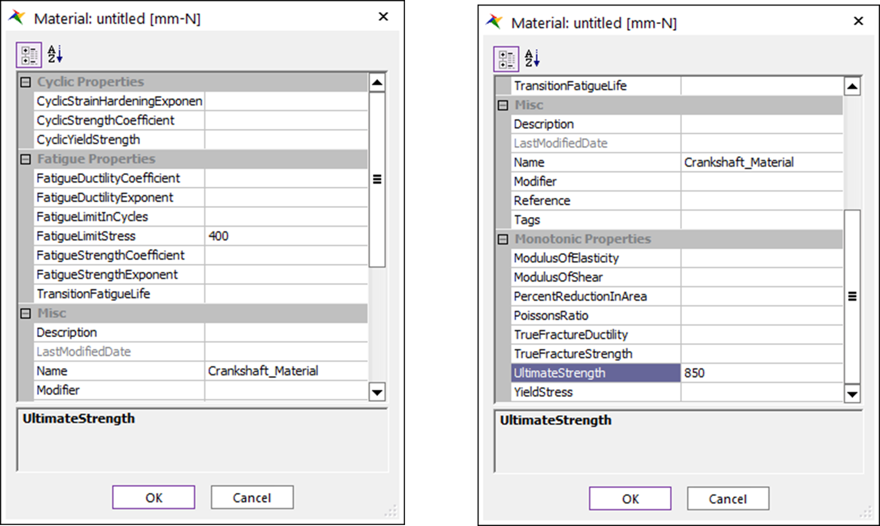
3. In the dialog window to create the new material, perform the following:

   • For the FatigueLimitStress value, enter 400.

   • For the Name, enter Crankshaft_Material.

   • For the UltimateStrength, enter 850.

   • Click OK.

     

   Tip

   The material property information required to derive the safety factor is the fatigue limit stress and the ultimate strength. However, the fatigue limit stress is not available in the material property information provided by the material library. In such cases, the cyclic yield stress is used instead of the fatigue limit stress information to derive the safety factor. However, when creating a new material to calculate the safety factor in this case, enter the fatigue limit stress directly.

4. Return to the Material Manager dialog window, right-click the newly created Crankshaft_Material and click Make Active.

5. In the Material Manager dialog window, click OK.

   

6. In the Fatigue Evaluation dialog window, click Calculation.

7. The safety factor is calculated again, as shown below. The fatigue limit stress and the yield stress of the new crankshaft material are much greater than those of [Steel] 1020. Therefore, the minimum safety factor result is larger than that of the previous result.

   

8.4.4.3.7. To reset the patch set and derive the safety factor again:

In the previous procedure, you derived the safety factor by selecting the patch set for the entire surface of the RFlex body. Consequently, the calculation takes a considerable amount of time. You can decrease the calculation time by only performing the fatigue analysis on specific sections. Choose these sections based on the Von-Mises stress contour results, and set the patch set only for those specific sections. To do so, follow these steps:

1. Double-click the RFlexBody1 to enter RFlex Body Edit Mode.

2. From the Set group in the RFlex Edit tab, click the Patch Set function.

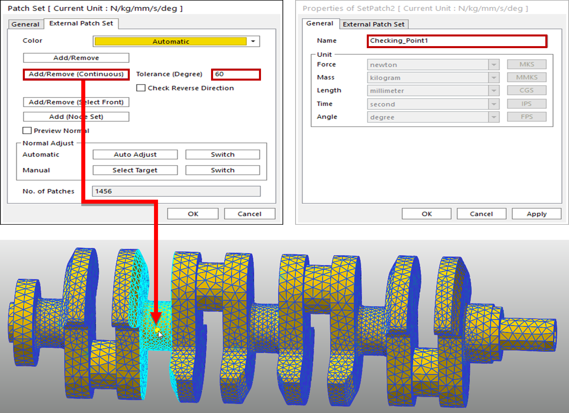
3. In the Patch Set dialog window, perform the following:

   • For the Tolerance (Degree), enter 60.

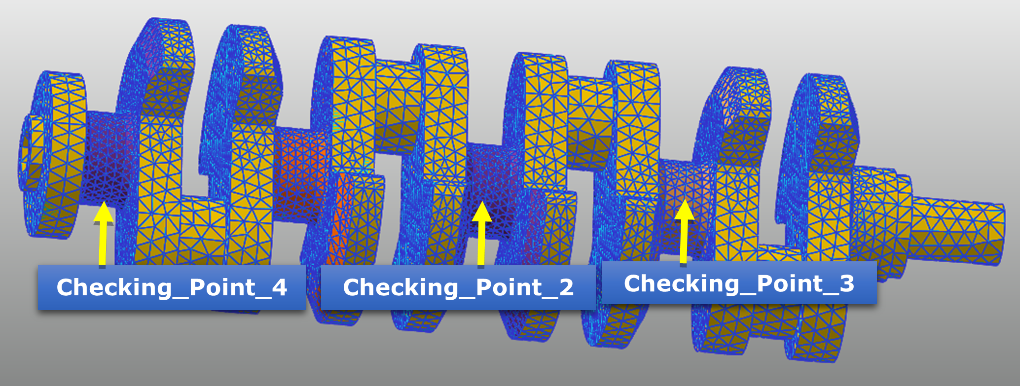
   • Click Add/Remove (Continuous), and select an element of interest, as shown below.

   • If the degree difference between the Normal Vectors of the selected patch and neighboring patches are within the range of 60 degrees, then the system automatically selects it as the patch set.

   • Right-click the element and click Finish Operation in the context menu.

   • On the General page, change the name to Checking_Point_1.

     

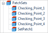
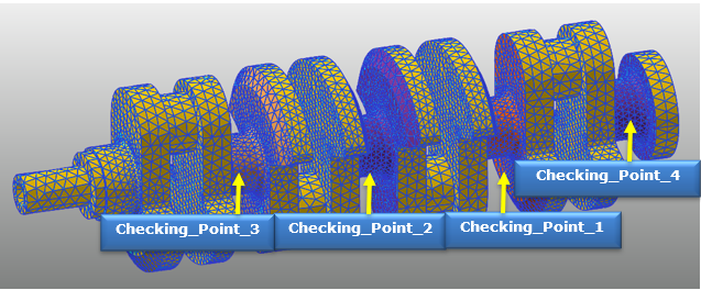
4. Repeat step 3 to create three more patch sets, as shown below. At this point, the names of the patch sets should be Checking_Point_2, Checking_Point_3, and Checking_Point_4.

   

5. After you have created the four patch sets, you can view the patch set information in the database, as shown in the figure to the below:

   

6. Confirm that the patch sets were created successfully, and then click the Exit function from the Exit group in the RFlex Edit tab to return to the parent mode.

7. From the Animation Control group in the Analysis tab, click the Reload the last animation file function.

8. From the Durability group in the Durability tab, click the Fatigue Evaluation function.

9. When the Fatigue Evaluation dialog window appears, change the name of the Element/Patch Set to Crankshaft.Checking_Point_1. Do not change any other settings.

   

10. Click Calculation to produce the calculation results.. Note that the calculation time is much faster than before.

11. Click OK.

12. From the Durability group in the Post Analysis tab, click the Contour function.

13. In the Contour dialog window, click Calculation.

14. Click Contour View to show the result for Checking_Point_1, as shown below.

    

15. Perform the same procedure to get the results for Checking_Point_2, Checking_Point_3, and Checking_Point4.

8.4.5. Analyzing and Reviewing the Results

8.4.5.1. Task Objective

This chapter teaches you how to analyze and review the safety factor results of the model.

8.4.5.2. Estimated Time to Complete

10 minutes

8.4.5.3. Analyzing the Safety Factor Results

The fatigue results from the durability analysis include the safety factor and the fatigue life. In general, a safety factor represents the relationship between the maximum stress and the allowable stress. However, the safety factor in the fatigue analysis indicates a different relationship.

• As shown below, the straight (Goodman method) and parabolic (Gerber method) equations for the relationship between the fatigue limit stress and the ultimate strength produce the minimum safety factor using the Rainflow Counting results (mean stress, stress amplitude) necessary for durability analysis.

  

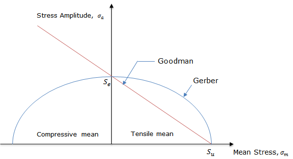
• Therefore, the fatigue limit stress and the yield stress are sufficient to derive the safety factor. In this tutorial, you have also used these two data items to derive the safety factor of the crankshaft material created during the new material creation process.

• The first durability analysis performed in this tutorial took approximately 2 minutes to create the patch sets for the entire RFlex body and derive the safety factor (this time may vary depending on your PC specifications). This may seem like a relatively long time, but it can be decreased as follows:

  1. Study the Von-Mises stress distribution in the RFlex/Contour and identify the weak sections of the structure.

  2. Set the patch sets for the weak sections only.

  3. This method is essential if you need to derive fatigue results repeatedly while varying the durability analysis conditions.

     

• The following table compares the safety factors derived from the four patch sets for the initially chosen material ([Steel] 1020) and the new crankshaft material.

  Material Patch Set	Minimum Safety Factor
  	Crankshaft material	[Steel] 1020
  Checking_Point_1	7.155	4.309
  Checking_Point_2	12.813	8.349
  Checking_Point_3	7.763	4.619
  Checking_Point_4	3.331	2.188

• Since the proportional limit and the yield stress for the new crankshaft material are greater than those for [Steel] 1020, the new crankshaft material has a higher safety factor. Furthermore, you can see that the section where the smallest safety factor is derived from is Checking_Point_4.

• In general, the Safety Factor in a structure can be expressed by the relationship between the maximum stress and the yield stress. Assuming the maximum stress at Checking_Point_4 of the crankshaft used in this tutorial is 72 Mpa and the yield stress of [Steel]1020 is 262 Mpa, then the safety factor could simply be expressed in 262/72=3.63. However, the result you got in this tutorial is 2.188, and you can see that there is a difference.

• If the crankshaft does not get dynamic loads in the engine but gets only static loads, then it is significant to derive the safety factor with the yield stress and the maximum stress. However, when it is the structure exhibiting dynamic behaviors such as the crankshaft, the safety factor derived from fatigue analysis does become significant.