10.2. Styler (Flex – Particleworks)
10.2.1. Overview
This tutorial covers how to perform co-simulation between RecurDyn and Particleworks. In this tutorial, co-simulation is performed on the dynamic interaction between the flexible bodies of RecurDyn and the fluid particles of Particleworks.
The model that will be covered in this tutorial is the Styler mechanism. The Styler is used to shake off the dust attached to cloth and to remove its wrinkles with steam. This tutorial analyzes the dynamic interaction between the clothes, which is expressed as a flexible body, and the steam, which is expressed as particles. After the co-simulation, we will also check the stress formed as the particles touch the flexible body, using the Contour function of RecurDyn.
10.2.1.1. Task Objectives
This tutorial covers the following topics:
How to export *.wall files of rigid and flexible bodies in a RecurDyn model
How to create particles in Particleworks
How to set fluid properties in Particleworks
How to perform co-simulation in RecurDyn
How to perform post-processing in RecurDyn
10.2.1.2. Prerequisites
This tutorial is intended for users who have completed the basic tutorials provided with RecurDyn. If you have not completed these tutorials, then you should complete them before proceeding with this tutorial.
Particleworks software must be installed to proceed with this tutorial. This tutorial was created based on Particleworks 7.1.0.
In this tutorial, the analysis was carried out using the NVIDIA GeForce GTX TITAN graphics card. Depending on the specifications of the computer and the version of the software, there may be slight differences in the results of the analysis.
10.2.1.3. Procedures
Procedures |
Time (minutes) |
Registering Particleworks GUI on the RecurDyn ribbon |
10 |
Modifying a RecurDyn Model |
10 |
Creating a Particleworks Model |
15 |
Co-simulation |
10 |
RecurDyn Post-processing |
5 |
Total |
50 |
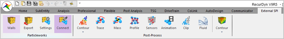
10.2.2. Register Particleworks GUI in RecurDyn
By default, the External SPI (Particleworks) GUI is not visible in the RecurDyn. You must add the GUI to RecurDyn using the configuration XML file provided by Particleworks.
10.2.2.1. Task Objective
Learn how to register External SPI(Particleworks) tab in RecurDyn ribbon using the configuration XML and to set a particle solver DLL.
10.2.2.2. Estimated Time to Complete
10 minutes
10.2.2.3. Copy Configuration XML
10.2.2.3.1. To copy Particleworks.xml:
10.2.2.3.2. To paste XML in RecurDyn:
10.2.2.3.3. To confirm RecurDyn GUI:
Run RecurDyn and check a ribbon GUI, you can see the External SPI tab and there is a Particleworks group.
10.2.2.3.4. To check a path of particle solver DLL:
Must check where particle solver DLL file should be located.
From the Paticleworks group in the External SPI tab, click the Settings function.
In the Settings dialog box, click the Info.
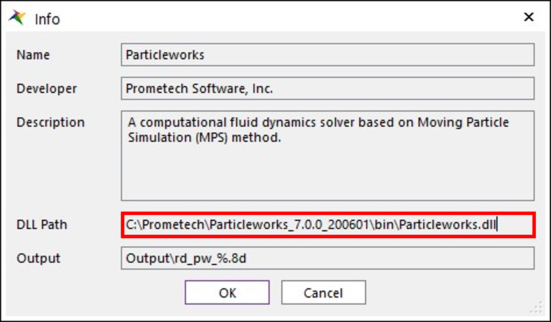
You can check the DLL Path in the Info dialog window. This path is set to the default installation location of Particleworks. So, if you installed Particleworks in a different path, you must modify the DLL path in the Configuration XML file.
Tip
Modifying the Particle Solver DLL path in Configuration XML file
(Perform it when the DLL path in the Info dialog window is different from the Particleworks installation path.)
Open the Particleworks.xml file.
Modify the DLL path following <Path> as shown below.
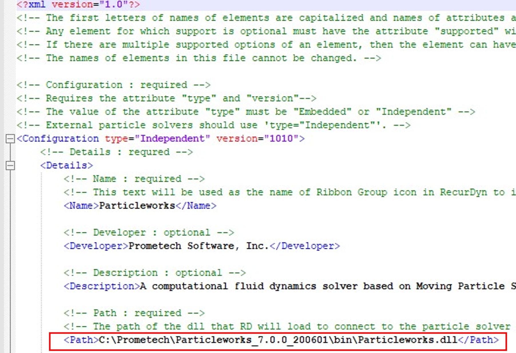
Save the Configuration XML file.
After confirming that the Configuration XML has been modified successfully, restart RecurDyn.
10.2.3. Modifying a RecurDyn Model
10.2.3.1. Task Objectives
In this chapter, you will learn how to create a flexible wall for analysis and how to export the necessary files in Particleworks.
10.2.3.2. Estimated Time to Complete This Task
10 minutes
10.2.3.3. Defining a patch set
For co-simulation between flexible bodies and particles of Particleworks, the portion of the flexible body that contacts the particles must be defined as a patch set.
Open the Styler_flex_model_cloth_start.rdyn file that was provided as an example model for this tutorial.
Enter Flex Edit Mode of the Cloth_FE body.
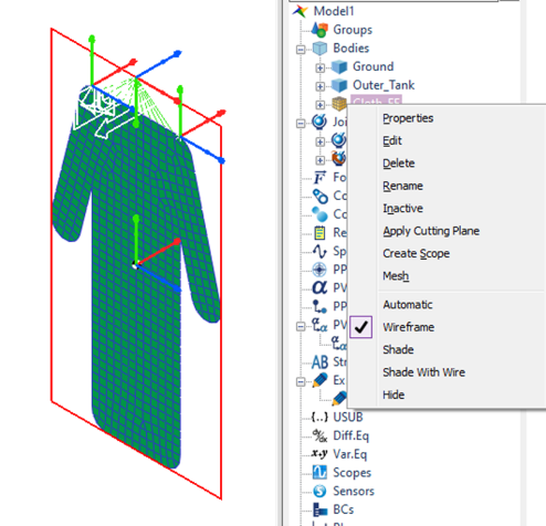
In the Set group of the FFlex Edit tab, click the Patch Set function.
When the Patch Set dialog box appears, click Add/Remove.
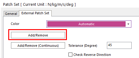
Select all patches by dragging them, right-click the mouse, and click Finish Operation.
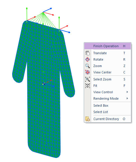
Click the OK button.
Exit the Edit mode.
10.2.3.4. Creating walls
Create walls for Outer_Tank and Cloth_FE.
In the Particleworks group of the External SPI tab, click the Walls function.
In the Working Window, click Outer_Tank.
Click Walls again, and click Cloth_FE.SetPatch1 in the Working Window.
Tip
You can select Cloth_FE by using Select Box or Select List, which are existing methods for selecting internal bodies. In this model, however, Outer_Tank is set as the layer 2 in a multi-layer. So, if you press Ctrl+2, which is a shortcut key combination for Layer hide/show, Outer_Tank will be hidden so that you can choose inner Cloth_FE more easily.
Modify the names of the walls as follows:
Wall1 Wall_Outer_Tank
Wall2 Wall_Cloth_FE
10.2.3.5. Exporting a *.wall file
In the Particleworks group of the External SPI tab, click the Export function.
- When the Export dialog box appears, locate the folder you want to save the file to and click OK to save it.The rd_pw.wall file and the WallGeometries folder are created in the saved folder. The files created in this chapter are moved to the Particleworks project folder in Chapter 4.
Tip
If you want to save the rd_pw.wall file somewhere else, you may do so. Pressing the Export button and clicking OK immediately saves the file in the default folder where the RecurDyn Model files are saved.Note
The rd_pw.wall file contains information about the position and orientation of wall geometries. If you import this file into Particleworks later, several wall geometries are imported at once. In the Wall Geometries folder, the files (*.obj or *.stl) related to wall geometry are automatically saved. Save and exit RecurDyn.
10.2.4. Creating a Particleworks Model
10.2.4.1. Task Objectives
In this chapter, you can import wall files from Particleworks and create fluid particles by using inflow as a model for steam.
10.2.4.2. Estimated Time to Complete This Task
15 minutes
10.2.4.3. Starting Particleworks
10.2.4.3.1. Create a new model
Double-click the Particleworks icon on the Desktop.
When you click Create Project on the File tab, the Create Project dialog box appears.
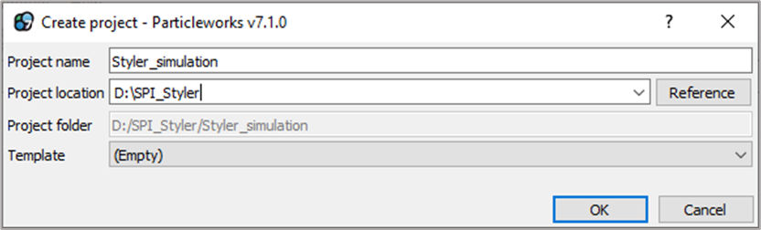
In the Project Name field, type Styler_simulation.
In the Project Location field, enter the location where the project will be created.
Click Finish to create the new model.
10.2.4.4. Configuring a preprocess
10.2.4.4.1. Import a wall file
Double-click the scene folder in the Projects dialog box.
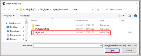
Click Import polygon files icon. The Open model files dialog box appears.
Click Open to import the rd_pw.wall file. <Project Location>\Styler_simulation\scene\rd_pw.wall
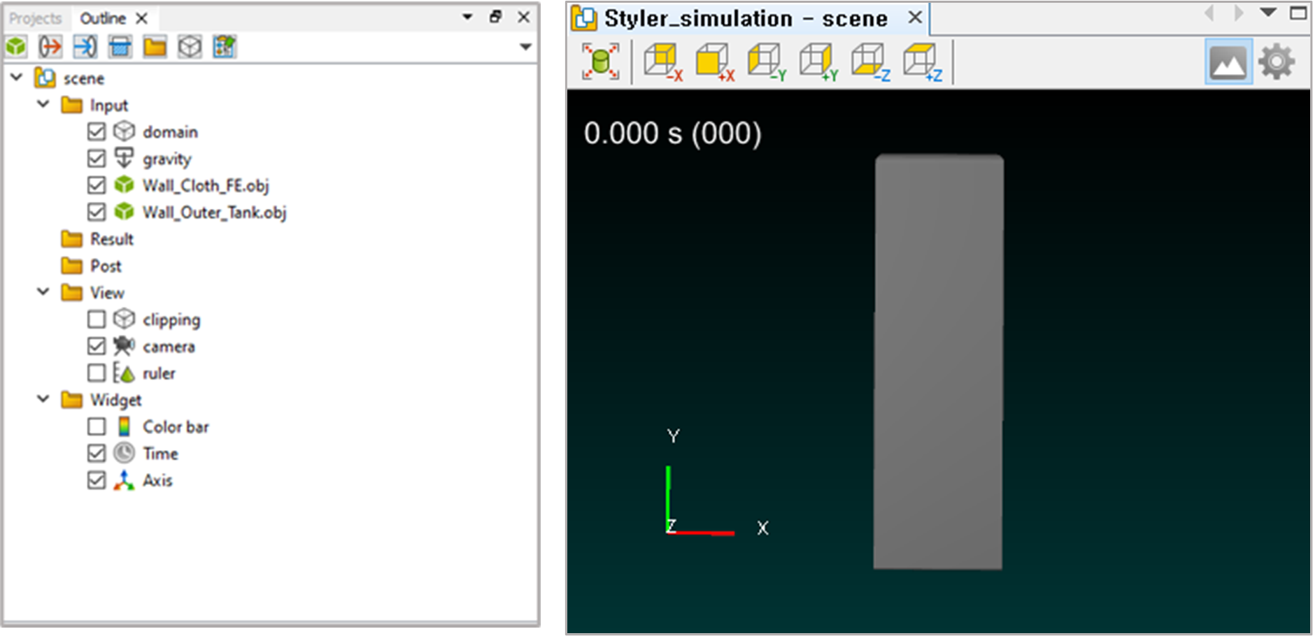
- Click the Fit button and the +Z plane button at the top of the Working Window to view the imported wall.As shown on the below, you can check whether the Wall_Cloth_FE.obj and Wall_Outer_Tank.obj are properly imported into the scene tree and check the shape of the imported wall files as shown on the below.
10.2.4.4.2. Set Wall_Outer_Tank.obj transparency
You need to adjust the transparency because the inner cloth is not visible due to Outer_Tank.
- In the Projects dialog box, click Wall_Outer_Tank.obj under scene > Input.The Properties dialog box associated with the entity you clicked is shown in the figure to the below scene tree.
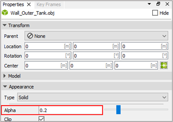
Change the Alpha value in the Appearance panel to 0.2 and press Enter.
Wall_Outer_Tank.obj becomes transparent, allowing you to look its inside.
10.2.4.4.3. Configure the camera
The default GUI setting of Particleworks is Turn Table, which is inconvenient to use. Switch the setting to a Track ball so that you can rotate it conveniently.
- In the Projects dialog box, click Camera under scene > View.The properties dialog box associated with the entity you clicked is shown in the figure to the below scene tree.
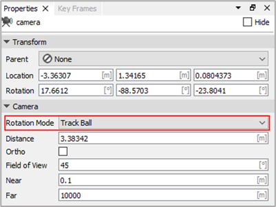
Change the Rotation Mode to Track Ball.
10.2.4.4.4. Set a domain
Domain is the area where fluid particles are analyzed. When the particles used as the steam fall down to the bottom, a reservoir at the bottom receives the water particles in the actual Styler. However, this analysis does not need to simulate the particles entering the reservoir. So, we will use a domain to delete the particles that fall down to the bottom.
In the Projects dialog box, double-click a domain under scene > Input.
Set the size of the domain as follows.
Upper limit: 0.3, 1.96, 0.3
Lower limit: -0.3, 0.55, -0.3
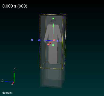

10.2.4.4.5. Create an inflow
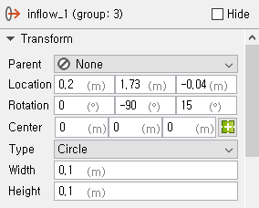
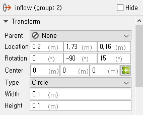
Inflow is a function that lets particles flow to the user-defined zone at the user-defined speed or flux.
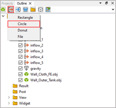
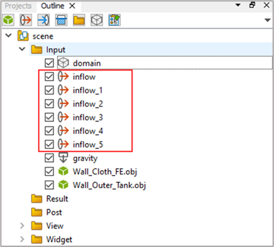
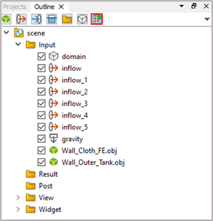
- Click the Circle button six times.In the Projects dialog box, six inflows are created in scene > Input.
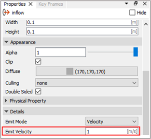
Click every inflow created in the Projects dialog box one by one to set the option values in the Properties dialog box as shown below.
Width and Height are set to the following values for all inflows.
Width: 0.1
Height: 0.1
inflow
Location: 0.2, 1.73, 0.16
Rotation: 0, -90, 15
Inflow_1
Location: 0.2, 1.73, -0.04
Rotation: 0, -90, 15
Inflow_2
Location: 0.2, 1.73, -0.24
Rotation: 0, -90, 15
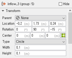
Inflow_3
Location: -0.2, 1.73, 0.24
Rotation: 0, 90, -15

Inflow_4
Location: -0.2, 1.73, 0.04
Rotation: 0, 90, -15
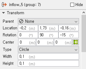
Inflow_5
Location: -0.2, 1.73, -0.16
Rotation: 0, 90, -15

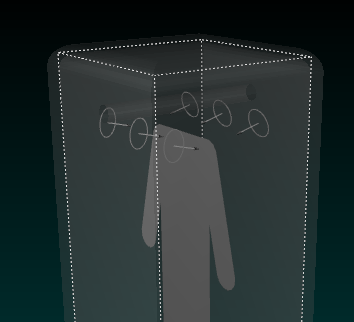
Confirm that the inflows are well defined as shown in the figure on the below.
10.2.4.4.6. Create and configure physical properties
At the top of the scene tree, click Manage physical properties….
- When the Physical property manager dialog box appears, click the + button to create a fluid.The basic physical property of the generated fluid is water. So you can use it as is.
- Click the + button again to create a polygon.Polygon is a physical property that specifies the rigid or flexible body defined as a wall by RecurDyn.
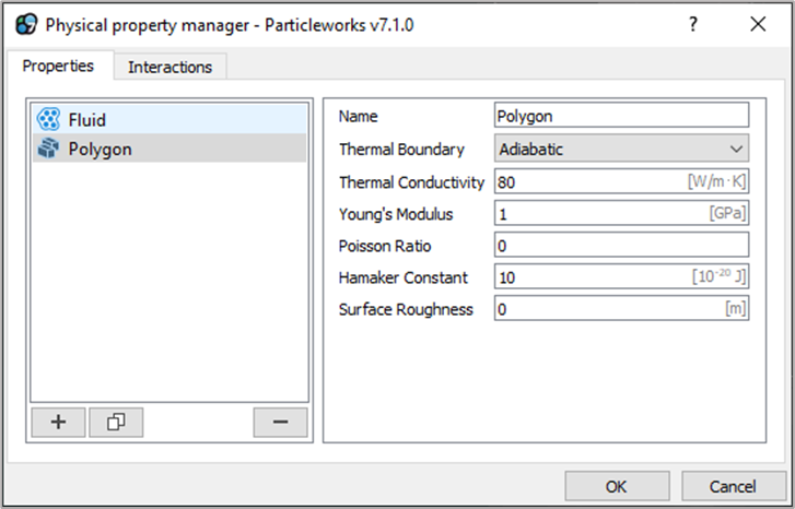
Click OK to close the dialog box.
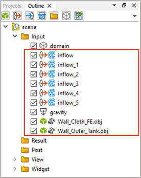
In the Scene tree, change the physical properties from None to the values specified below.
Wall_Cloth_FE.obj: Polygon
Wall_Outer_Tank.obj: Polygon
All inflows: Fluid
In the Properties tab of every inflow, set the value for Emit Velocity as shown below.
Emit Velocity: 1
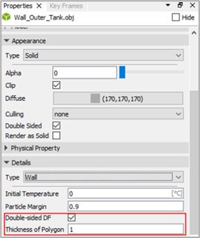
In the Properties tab of Wall_Cloth_FE.obj, check Double-sided DF and set the Thickness of Polygon as follows.
Thickness of Polygon:1
10.2.4.4.7. Configure particles and preferences
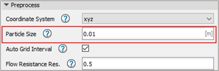
Click the Setting icon, and change options of Basics tab in Run dialog.
In the Particle Size field, enter 0.01.
Note
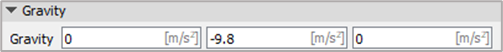
In the case of SPI, the unit in Particleworks must be set to meter regardless of the unit in RecurDyn.If the unit in RecurDyn is set to meter, you don’t need to convert the particle size or domain size and you just need to use the same values in Particleworks. If the unit in RecurDyn is set to millimeter, you need to convert the millimeter values to the meter values and enter the meter values in Particleworks.In the Y field of the Gravity pane, enter -9.8, just like in RecurDyn.
Click the Next button, and Set the Viscosity option as shown below in MPS tab.
Type: Implicit
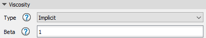
Leave the others at the default settings and click Next.
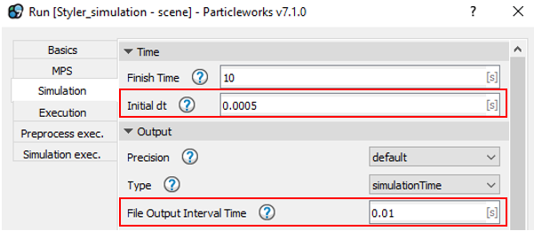
10.2.4.4.8. Configure analysis conditions
Set the analysis options in the Run dialog box.
In the Time pane, enter 0.0005 in the Initial dt[s] field.
Enter 0.01 in the File Output Interval Time[s] field.
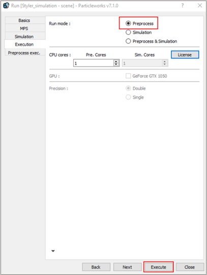
10.2.4.4.9. Create particles
In the Run dialog box at Execution tab, set the Run mode option to Preprocess.
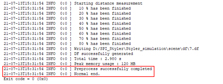
- Click Execute.If the message saying that the particle creation is completed appears in the Output dialog box as shown below, the particles have been created.
10.2.4.5. Preparing for Co-simulation
To do co-simulation in RecurDyn, you need to create some files in Particleworks. The relevant files are automatically generated by Particleworks as you go through the standalone analysis.
Perform standalone analysis in Particleworks.
On the Simulation tab, click Run.
At Execution tab, Set the Run mode option to Simulation.
Enter the number of CPU cores to be used for the analysis. If there is a GPU, select the GPU to be used for the analysis.
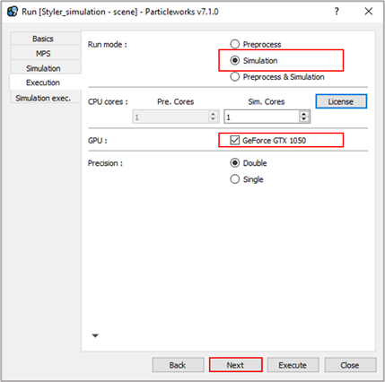
Click Next.
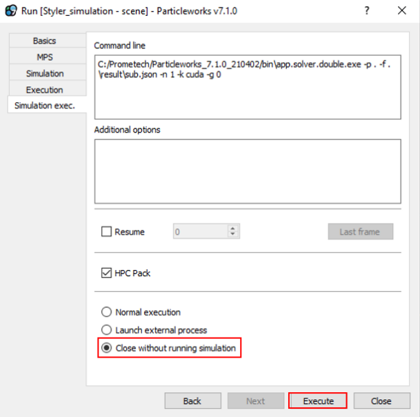
Check Close without running simulation.
Click Execute.
Save the project.
The Particleworks program may be turned off in Chapter 5. However, in this tutorial, we will proceed to the next chapter with the program turned on to check the analysis results in real time during analysis.
10.2.5. Co-simulation
10.2.5.1. Task Objectives
In this chapter, we will perform co-simulation using RecurDyn and Particleworks to analyze the interaction between flexible bodies and particles.
10.2.5.2. Estimated Time to Complete This Task
10 minutes
10.2.5.3. Co-simulation
10.2.5.3.1. Perform co-simulation in RecurDyn
- Run RecurDyn and open the Styler_flex_model_cloth_start.rdyn file you copied.(The file path: <ProjectLocation>\Styler_simulation\scene\Styler_flex_model_cloth_start.rdyn)
In the Simulation Type group of the Analysis tab, click the Dynamic / Kinematic Analysis function to open the Dynamic/Kinematic Analysis dialog box.
Check the simulation end time and step.
End Time: 1
Step: 500
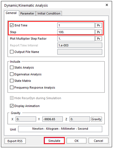
Click Simulate to perform the analysis.
Tip
Some of the options in the Dynamic/Kinematic Analysis dialog box are as follows.
End Time: Defines the simulation duration.
Step: Defines the number of frames that are saved during the entire simulation duration.
Plot Multiplier Step Factor: Defines the number of saved data points for plotting. The number of plot data points is defined by multiplying Step by Plot Multiplier Step Factor.
Tip
Set RPA Setting option in Particleworks Setting dialog
Before proceeding co-simulation, user needs to use TranslationalVelocity, the data of RPA file, which is the output of the particle, for contour.
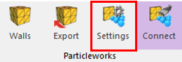
Click the Settings function in External SPI tab.
Check Use option of TranslationalVelocity in RPA Settings.
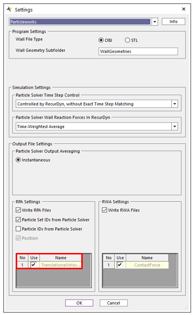
Click OK Button.
10.2.6. Checking the Analysis Results
10.2.6.1. Task Objectives
In this chapter, we will check how particles affect a flexible body using Contour.
10.2.6.2. Estimated Time to Complete This Task
5 minutes
10.2.6.3. Checking Contour
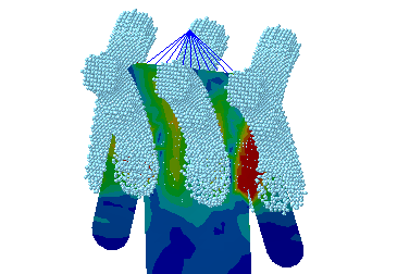
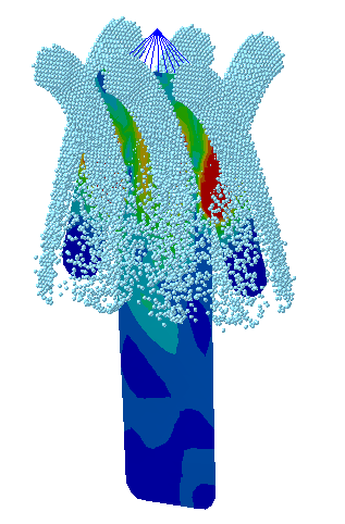
After the analysis is completed, you can check the result using Contour to see whether the particles affect the flexible body. And since we do not actually model the exact physical properties and interactions of the fabric, the values from the stress or reaction force are not exact experimental values. So please check only whether the flexible body is affected by the particles.
In the FFlex group of the Flexible tab, click the Contour function.
In the Contour dialog box, set the Type to User Defined and click Calculation.
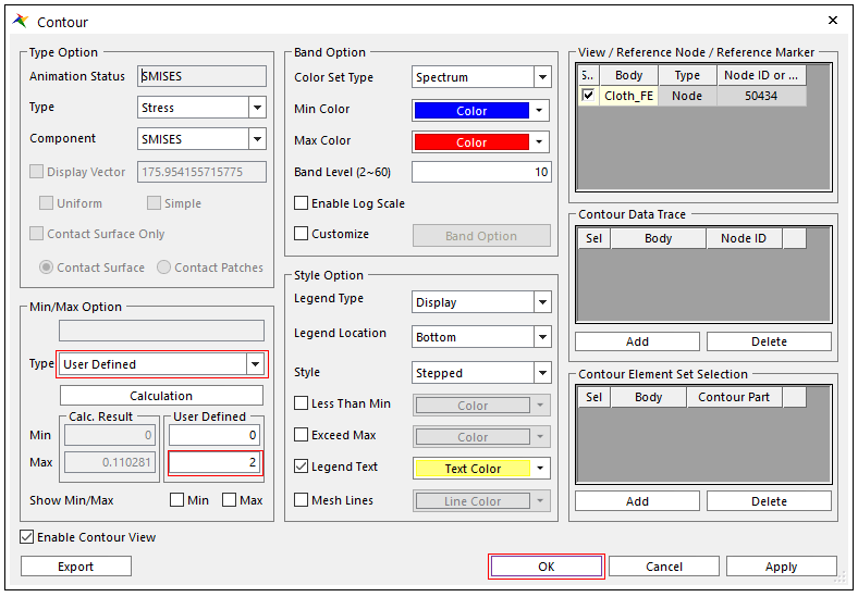
Change the Max value of User Defined to 2 and click OK.
In the Animation Control group of the Analysis tab, click the Play function to see Contour.