8.2. FFlex ConnectingRod Tutorial (Durability)

8.2.1. Getting Started

8.2.1.1. Objective

The modeling and simulation of flexible bodies within a multibody dynamic system is an important capability that enables users to obtain more accurate results from their simulations. RecurDyn offers two methods to do this: Reduced Flex (RFlex) and Full Flex (FFlex). RFlex can quickly simulate models where there are well-defined attachment points where the other bodies connect to the flexible body, where there is no contact with the flexible body, and where deformation is small and within the linear range. FFlex, on the other hand, can handle rolling and sliding contact with the flexible body, as well as large deformations of the flexible body which exhibit nonlinear behavior.

Once a flexible part has been simulated during a single work cycle, the user can easily predict the lifetime of that part using RecurDyn/Durability. This fully integrated RecurDyn module seamlessly transfers dynamic analysis results into a fatigue analysis, allowing the user to choose from dozens of fatigue models most commonly used in industry to predict fatigue life. Also included is a fatigue material library containing 180 common materials based on the SAE J1099 technical report.

The example used in this tutorial will be the connecting rod in a four-cylinder engine. This component, for obvious reasons, goes through many cycles of loading from the combustion force produced in the piston chamber.

8.2.1.2. Audience

This tutorial is intended for intermediate users of RecurDyn who have previously learned how to model flexible bodies using RecurDyn/FFlex. All new tasks are explained carefully.

8.2.1.3. Prerequisites

Users should first work through the 3D Crank-Slider, Engine with Propeller, and Pinball (2D contact) tutorials, or the equivalent, followed by the FFlex Compliant Clutch tutorial. We assume that you have a basic knowledge of physics.

8.2.1.4. Procedures

The tutorial is comprised of the following procedures. The estimated time to complete each procedure is shown in the table.

Procedures	Time (minutes)
Review the FFlex model setup and dynamic simulation results	10
Perform the fatigue analysis and view results	20
Total	30

8.2.1.5. Estimated Time to Complete

This tutorial takes approximately 30 minutes to complete.

8.2.2. Reviewing the Model Setup

8.2.2.1. Task Objective

Learn about the model and the special considerations made for the flexible connecting rod.

8.2.2.2. Estimated Time to Complete

10 minutes

8.2.2.3. The Engine with Flexible Connecting Rod Model

The model being used in this tutorial is a traditional internal combustion engine with one of the connecting rods modeled as a RecurDyn/FFlex flexible body.

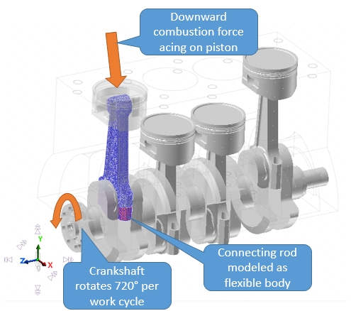
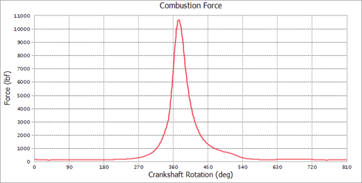
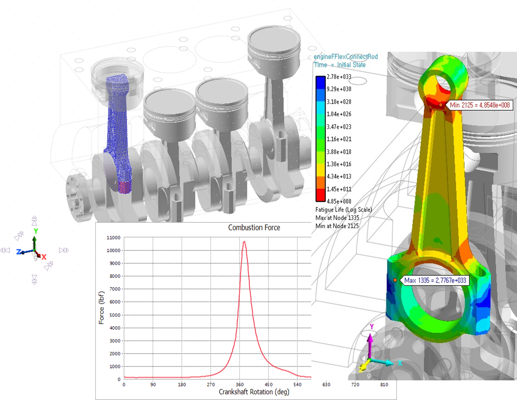
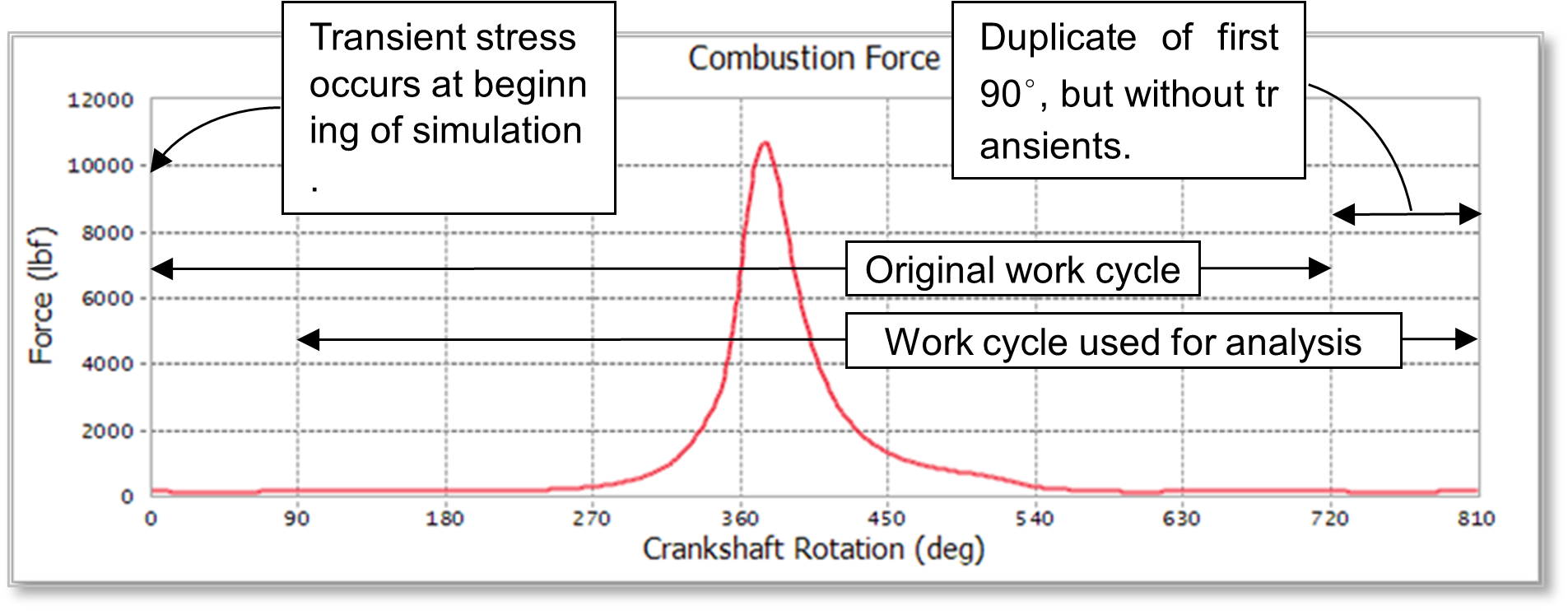
The combustion force, as shown on the upper figure, has a large peak shortly after 360° of crankshaft rotation. A full cycle is completed after the crankshaft rotates 720°. For reasons to be described later, the dynamic simulation of this model runs for slightly longer, allowing the crankshaft to rotate 810°. At 3,000 RPM, this takes 0.045 sec.

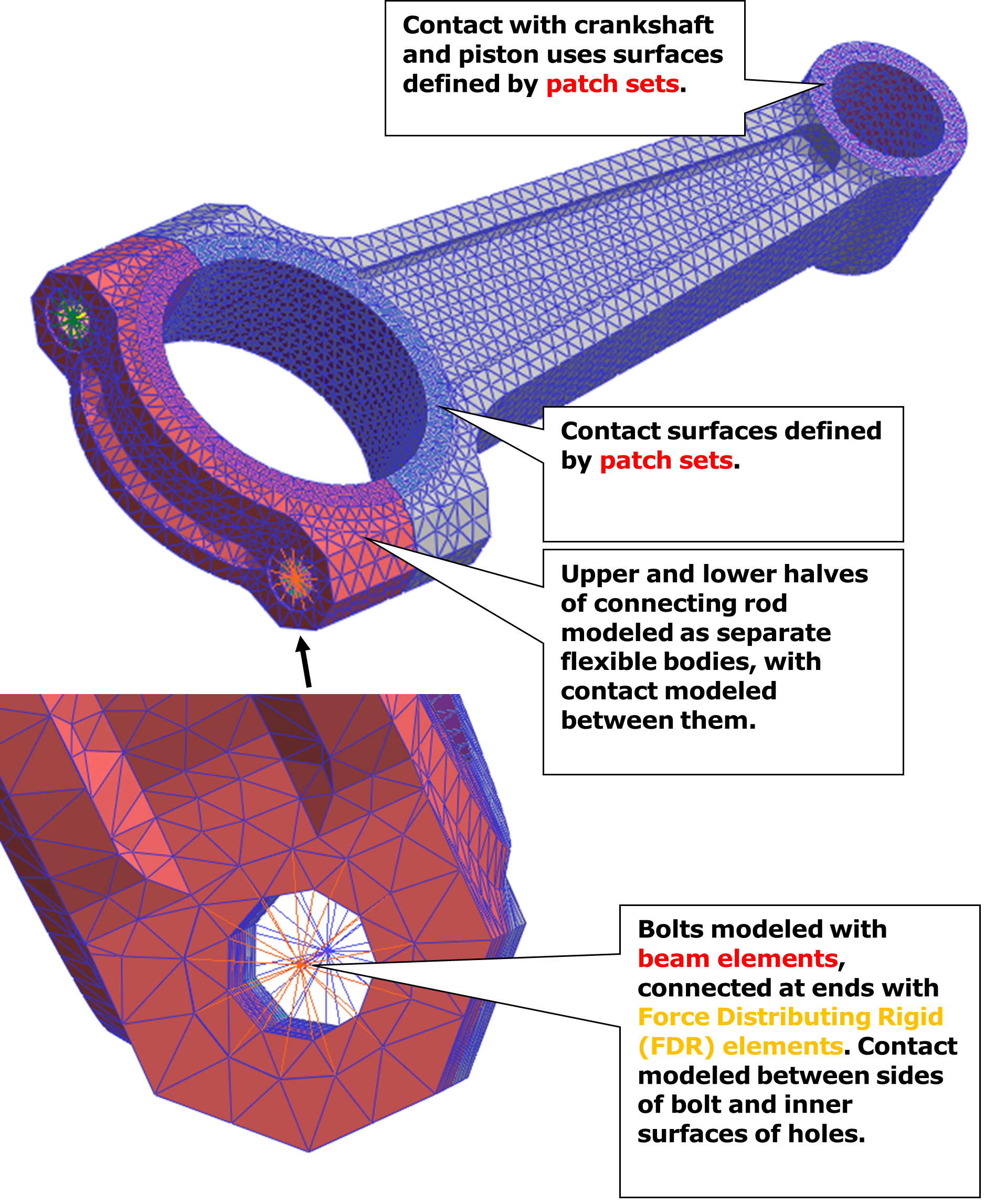
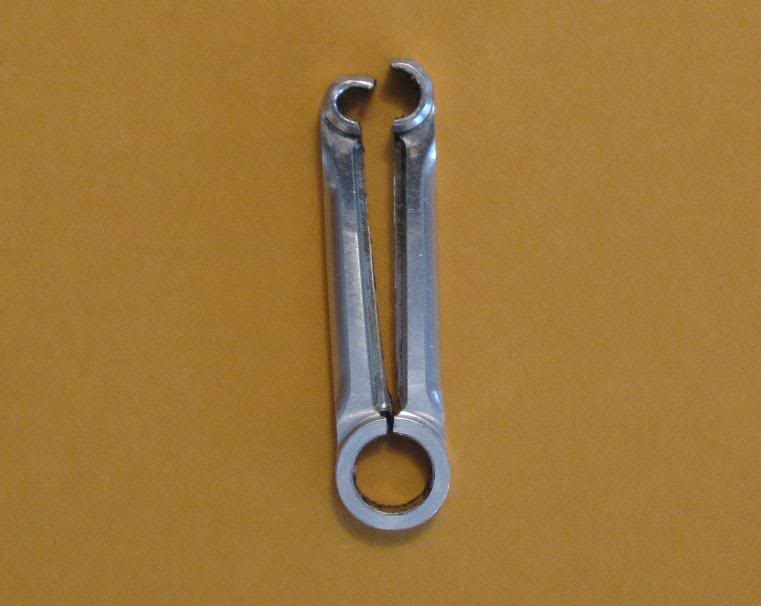
Shown below is the FFlex connecting rod. For the purpose of this tutorial, the meshing is coarser than what would be recommended to get the most accurate results. To more accurately reflect reality, the connecting rod has been meshed as two separate parts connected with two bolts. Contact between the upper and lower half has been modeled. The bolts are attached at the ends using Force Distributing Rigid (FDR) elements, which are analogous to RBE2 elements, and contact with the bolts has been modeled as well.

When connecting this body to the crankshaft and piston, no joint entities were used (i.e. revolute joints). Instead, only contacts were modeled between the flexible body and the other bodies it interacts with. The importance of including this level of fidelity can be seen in the following figure.

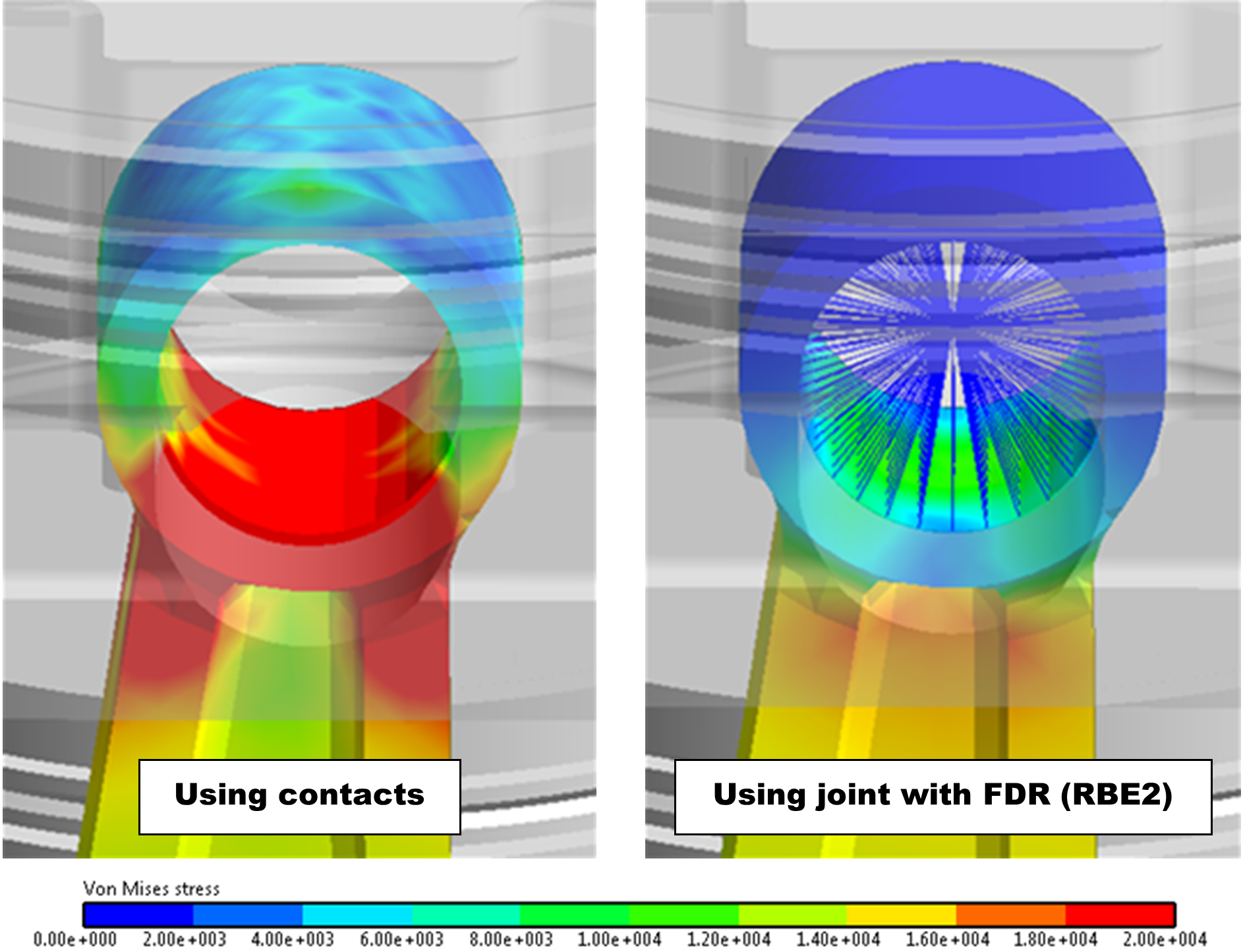
The two images above are the results from the two separate but similar simulations. In both simulations, the image was taken when the combustion force is at its peak, exerting a downward force onto the piston and subsequently the connecting rod. In one simulation, only contacts were used to model connection between the piston and the connecting rod. Here, the contact allows the force to realistically be applied mainly to the bottom of the cylindrical surface. As a result, the Von Mises stress is concentrated in the bottom and not in the upper part of the surface. In the other simulation, a revolute joint was used instead, along with a Force Distributing Rigid (FDR) element (similar to and RBE2 element) which is used to distribute the joint load across the multiple nodes. In this situation, the FDR introduces an artificial stiffness into the structure, which reduces the amount of internal stress in the whole area around the joint.

Therefore, in this tutorial, we use the FFlex model which was defined several contacts between the piston and the connecting rod in order to check the fatigue life on the area with high stresses.

8.2.2.4. Reviewing the Dynamic Simulation Results

You will now adjust the FFlex contour plot settings and play the animation of the results to observe when and where high stress occurs in the connecting rod throughout a single work cycle.

8.2.2.4.1. To view the dynamic simulation results:

1. Start RecurDyn and open the engineFFlexConnectRod.rdyn model.

   (The file path: <InstallDir>\Help\Tutorial\PostAnalysis\Durability\FFlexConnectingRod).
2. From the File menu, click Save As.

   (Save this model in the different path because it is impossible to simulate directly in the tutorial path.)

3. From the Simulate Type group in the Analysis tab, click the Dynamic/Kinematic Analysis function push the Simulate on the Dynamic/Kinematic Analysis dialog after the Dynamic/Kinematic Analysis dialog box appears.

4. From the FFlex group in the Flexible tab, Click the Contour function.

5. Make the following settings, so that they appear as shown below.

   

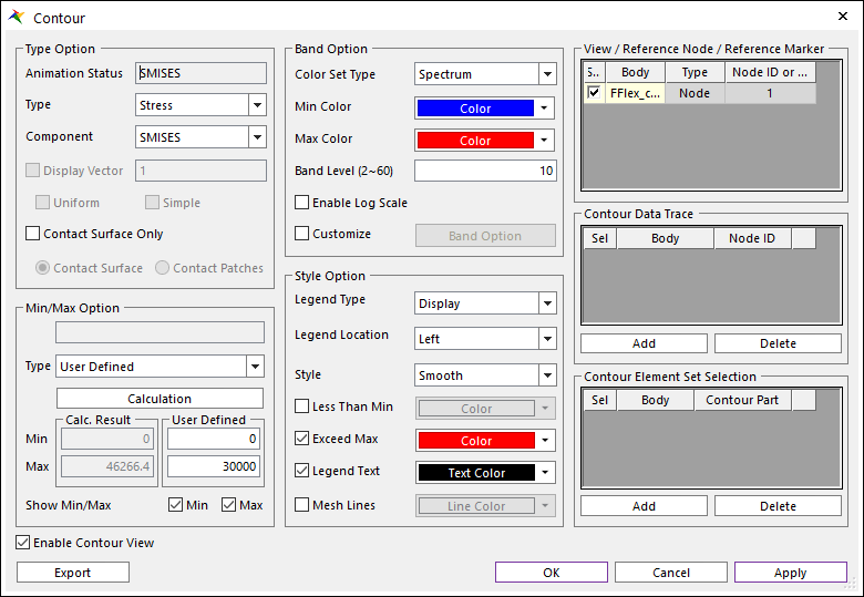
6. Click OK.

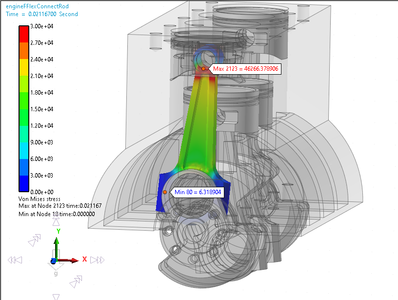
7. From the Animation Control group in the Analysis tab, Click the Play function.

You should see that the stress increases dramatically at about frame 382, when the combustion force peaks. If you were to adjust the maximum stress value on the scale to 30,000 (lbf/in^2), the contour plot would appear as shown at below.

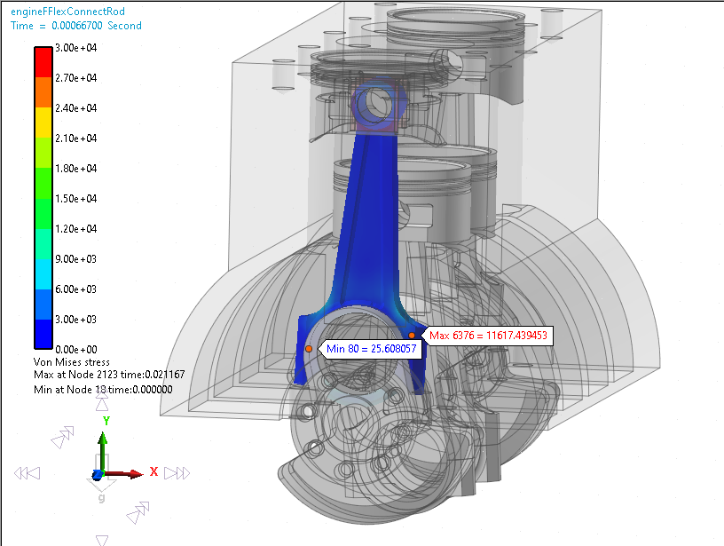
You might also have noticed that, at the beginning of the simulation, there are some initial transient stresses within the connecting rod that dissipate about frame 13. These stresses are concentrated in the areas where the connecting rod makes contact with the piston and the crankshaft. In this model, these transient effects are difficult to avoid because they are caused by the mechanism starting with a high initial velocity and the FFlex body’s initial velocity or acceleration not matching up exactly with that of the bodies it’s making contact with. However, for the fatigue analysis we can simply ignore these initial frames where the transient stresses occur so that they do not throw off the results, as described on the next page.

To avoid the transients while still capturing the first 90° of crankshaft rotation, the simulation end time has been extended to allow the crankshaft to rotate an extra 90° after it completes its 720° work cycle rotation. We can include this last 90° of rotation and use it in place of the first 90°, because it is a duplicate of the first 90° of rotation but without the transients caused by the beginning of the simulation.

8.2.3. Performing the Fatigue Analysis

8.2.3.1. Task Objective

Learn to:

• Create a patch set to define the fatigue analysis surface.

• Define the fatigue analysis preferences.

• Select a material from the included fatigue material library.

• Select the dynamic analysis data (animation frames) to be used in the fatigue analysis.

• Run the fatigue analysis and display contour plot results.

8.2.3.2. Estimated Time to Complete

20 minutes

8.2.3.3. Defining a Surface for the Fatigue Analysis

The fatigue analysis will be performed on the entire outer surface of the part. This is because part failure due to fatigue originates from the growth of cracks that have initiated on the surface. Selecting this subset of FFlex entities also reduces the computational requirements of the fatigue analysis by restricting the calculation to a set of faces smaller than the number of total elements.

To define the surface for fatigue analysis, you will create a patch set containing all the element faces that are on the surface of the part.

8.2.3.3.1. To create a patch set for the fatigue analysis:

1. Enter the Body Edit Mode for the FFlex_connectRod body.

2. Under the FFlex Edit tab, from the Set group, click the Patch Set function.

   
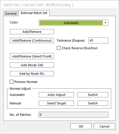
3. Set the Tolerance (Degree) to 90.

   With this setting, after the user selects a seed element face, RecurDyn will select any adjacent element face that forms an angle of up to 90 degrees with that initial face, and then select any element faces adjacent to and up to 90 degrees from those faces, etc. Because there is no edge in this part that is less than 90 degrees, all the outer faces will be selected.

4. Select Add/Remove (Continuous).

5. As shown in the following figure, first select a seed element face on the lower body of the connecting rod.

   
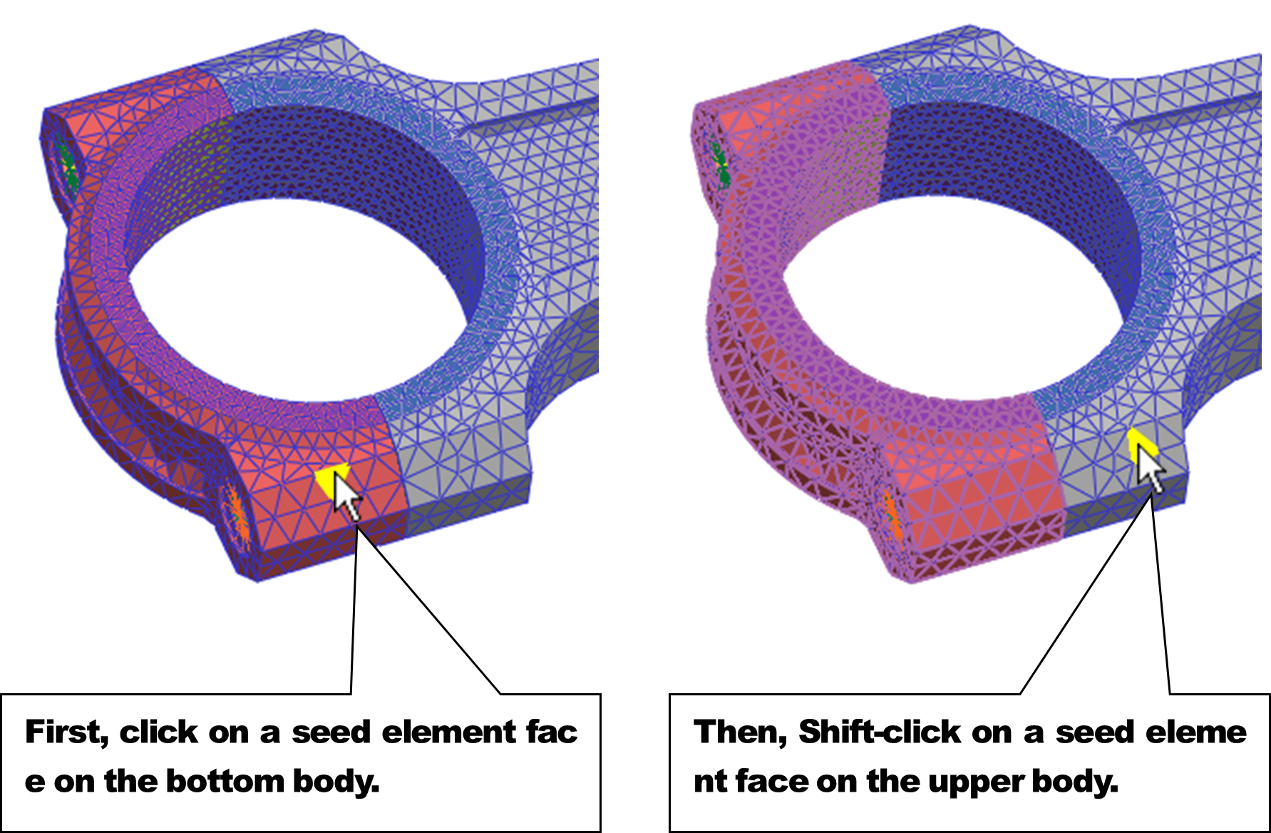
6. Next, hold the Shift key and click on a seed element face on the upper body.

   The element edges of both the upper and lower bodies should now be highlighted as shown below.

7. Right-click anywhere in the screen and select Finish Operation.

8. Click OK.

   There should now be a patch set which includes all the outer element faces of both the upper and lower bodies of the connecting rod.

9. Exit the body-edit mode and return to the top level of the model.

8.2.3.4. Setting Up and Running the Fatigue Analysis

Now that the fatigue analysis surface has been defined, the fatigue analysis can be run. However, because it relies on the results from the dynamic analysis, the animation must be imported again first. Note that the dynamic simulation does not have to be run again after defining the analysis surface.

8.2.3.4.1. To import the dynamic analysis animation data:

1. Click the Reload the last animation file function from the Animation Control group as shown in the figure below.

8.2.3.4.2. To set up and run the fatigue analysis:

1. From the Durability group in the Post Analysis tab, click the Preferences function.

2. Under the Material page, click … to set the location of the material library on your computer.

   
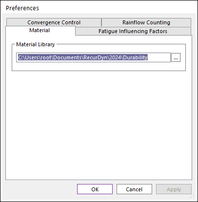
3. Navigate to the directory C:\Users\<Your Windows Login ID>\Documents\RecurDyn\<RecurDyn Version> (or equivalent, depending on your operating system)

   If you want to define the path to contain the Material Library, create a new directory called Durability and select it.

4. Select the Fatigue Influencing Factors page.

5. Set the Surface Factor (ms) to Machined.

   

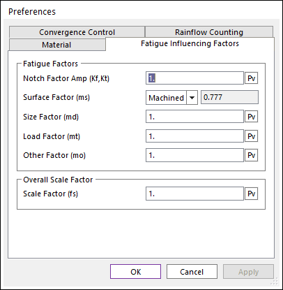
6. Click OK.

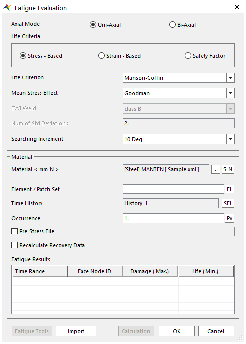
7. From the Durability group in the Post Analysis tab, click the Fatigue Evaluation function.

8. Ensure that the Axial Mode, Life Criteria, Mean Stress Effect, and Searching Increment are set as shown at below.

   (Especially, Axial Mode should be defined as Uni-Axial.)
   

9. Under the Material section, click … to select a material.

10. Scroll down to [Steel] 4130/258, right-click, and select Make Active.

    

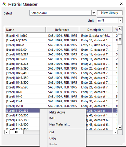
11. Click OK.

12. Back on the Fatigue Evaluation dialog, in the Element / Patch Set section, select EL.

13. From the Modeling Window, select the patch set that you had just created (FFlex_connectRod.SetPatch20).

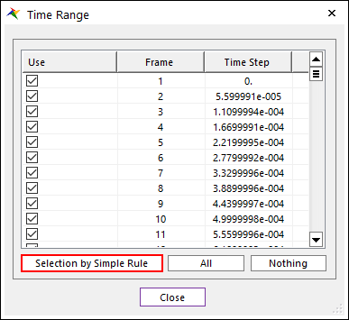
14. In the Time History (Frame) section, click the SEL button to make Time History sets and select which animation frames to include in the fatigue analysis in each set.

    

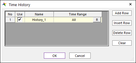
15. Modify the Name of Time History from History_1 to History_721.

16. Click R in the Time History dialog in order to change the time range.

17. Click Selection by Simple Rule.

    

18. Check the box next to Initialize before Update.

19. Make the following settings:

    • Start Index: 91

    • Increments in Index: 1

    • Number of Selections: 721

      

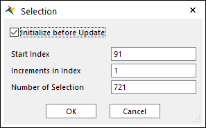
20. Click OK. And then, Close.

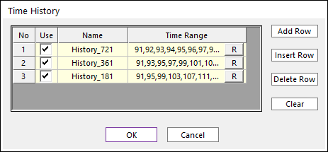
    • Click Add Row in Time History dialog, and then make other Time History whose name is History_361.

21. Perform the 17~ 19 procedure repeatedly, and then make the Time Range as follows.

    • Start Index: 91

    • Increments in Index: 2

    • Number of Selections: 361

22. Make another Time History set whose name is History_181, and Time Range is defined as follows.

    • Start Index: 91

    • Increments in Index: 4

    • Number of Selections: 181

23. Verify the defined Time History sets as shown the figure at the below and click OK.

    
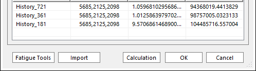
24. Back in the Fatigue Evaluation dialog, click Calculation.

    The fatigue analysis should perform three times and take about a few seconds to run. After that, the results are as shown at below.
    

25. Click OK.

8.2.3.5. Viewing the Fatigue Analysis Results

8.2.3.5.1. To view the fatigue analysis results:

1. From the Durability group in the Post Analysis tab, click the Contour function.

2. Make the settings as shown at below. Especially, Time History should be defined as History_721.

3. Under the Style Option section, next to Color Option, click Edit.

   

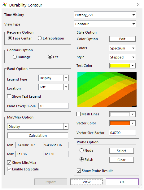
   Because you will be viewing the life data, you will want to switch the color options, so the color red is associated with lower values and blue with higher values.

4. As shown at below, select the minimum color as red and the maximum color as blue.

   

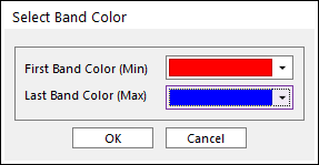
5. Click OK.

6. Click View. The results should appear as shown on the following page.

The results should appear as shown below. The area of lowest fatigue life, shown in red, occurs in the bottom edge of the hole where the piston attaches. The lowest life is 5.264e+08 cycles. If the engine were run under these conditions for 1 hour a day (90,000 ( = (1/0.04)*3600) ) cycle per 1 hour at 3,000 rpm, this would translate into a part lifetime of about 16 years.

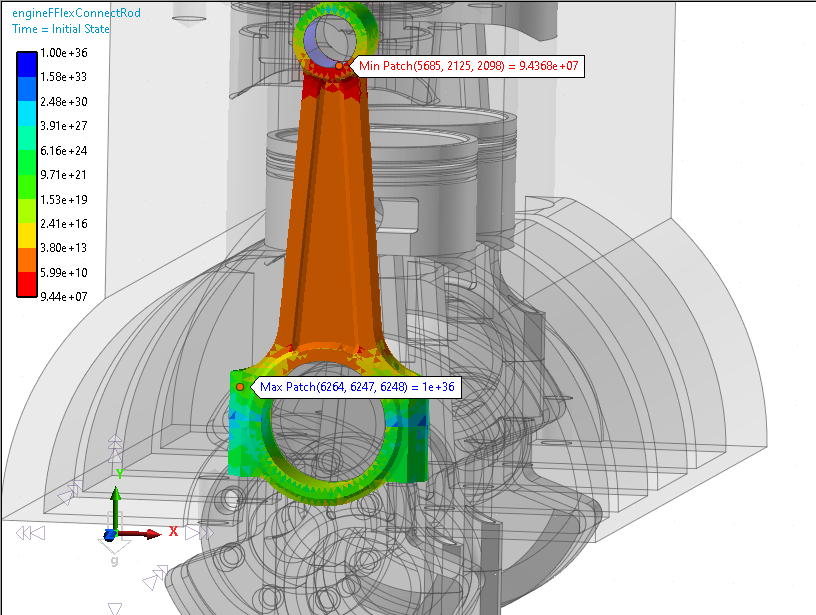
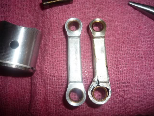
This failure location agrees with actual part failures that have occurred during operation. Once a small crack forms at the surface, it can propagate rapidly as shown below.

8.2.3.6. Ensuring Enough Frames are Selected

As mentioned earlier, the most accurate fatigue analysis results will be obtained if the most animation frames can be selected from the dynamic analysis. In addition, there is another way to check if enough frames have been selected to capture the behavior with enough resolution for the fatigue analysis. This method is to perform several fatigue analyses, each time increasing the number of selected animation frames until the fatigue analysis results converge.

For example, with the engine model, the table below shows the results obtained when selecting different numbers of frames. The difference between the minimum life results for 361 and 721 frames is exactly same. So, History_361 could be considered fairly well-converged.

Fatigue Life Results on the Contour Plot (% Difference from 721 Frame Results)
Frames	181	361	721
Time History	History_181	History_361	History_721
Minimum Life	1.0449e+08	9.8757e+07	9.4368e+07