6.1. Automotive Road Testing (TSG)

6.1.1. Overview

6.1.1.1. Task Objectives

In general, an actual vehicle drive test is used to obtain measurement data such as acceleration, speed and location from sensors for the vehicle part or system durability test. However, since measurement data are output signals derived from specific locations due to external actuation of the vehicle, it is hard to apply them as input signals of actuators in the actual vehicle test-rig or the virtual vehicle test-rig using RecurDyn. Moreover, since it is difficult to reflect all the nonlinear elements of the physical system in the virtual system modeled by RecurDyn, it is hard to assume both systems are identical. Therefore, if it is possible to derive input signals of actuators so that the measurement data can be derived from the RecurDyn modeling, you can resolve issues on the usability of measurement data and the reliability of the RecurDyn modeling. The TSG Toolkit uses the input signals of actuators included in the RecurDyn modeling for the measurement data to simulate actuation conditions of the physical system as similar as possible using the measurement data.

In this tutorial, the TSG Toolkit is used to generate input signals of actuators based on the measurement data obtained from the vehicle drive test.

• Configure sensors to utilize measurement data and to check the simulated result.

• Configure actuators to derive sensor results through simulation.

• Generate input signals of actuators to derive measurement data from sensors through simulation iteration.

  • Output signal derived from the sensor: Response signal

  • Output signal to be derived from the sensor (measurement data utilization): Target signal

  • Input signal of the actuator: Drive signal

• Check the result to see if the result derived from the sensor (response signal) and the measurement data (target signal) are similar.

6.1.1.2. Prerequisites

This tutorial is intended for users who have completed the basic tutorials provided with RecurDyn. If you have not completed these tutorials, then you should complete them before proceeding with this tutorial.

6.1.1.3. Procedures

This tutorial consists of the following tasks and the time required for each task is listed in the table below.

Procedures	Time (minutes)
Opening the initial Model	10
Defining Signals	10
Performing FRF	10
Performing Iteration	10
Total	40

6.1.1.4. Estimated Time to Complete this Task

40 minutes

6.1.2. Opening the Initial Model

6.1.2.1. Task Objectives

To open and observe the initial model.

6.1.2.2. Estimated Time to Complete This Task

10 minutes

6.1.2.3. Opening the RecurDyn Model

6.1.2.3.1. To run RecurDyn and open the initial model

1. On the Desktop, double-click the RecurDyn icon to open RecurDyn. When the Start RecurDyn dialog window appears, close it.

2. In the File menu, click the Open function.

3. Navigate to the tutorial folder and select TSG_Tutorial_Car_Start.rdyn.

   (File path: <InstallDir>\Help\Tutorial\TSG\AutomotiveRoadTesting)

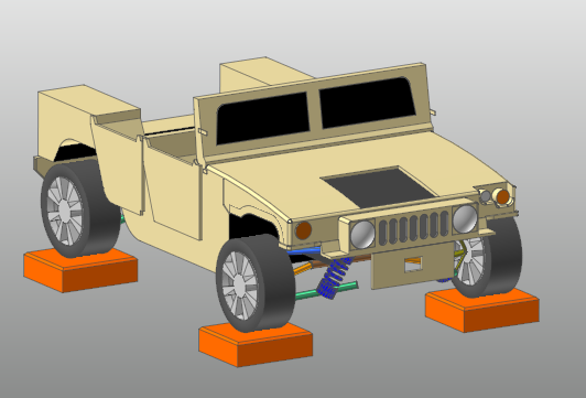
4. Click Open. to open the model shown in the following figure.

   

The following explains the configuration of the model.

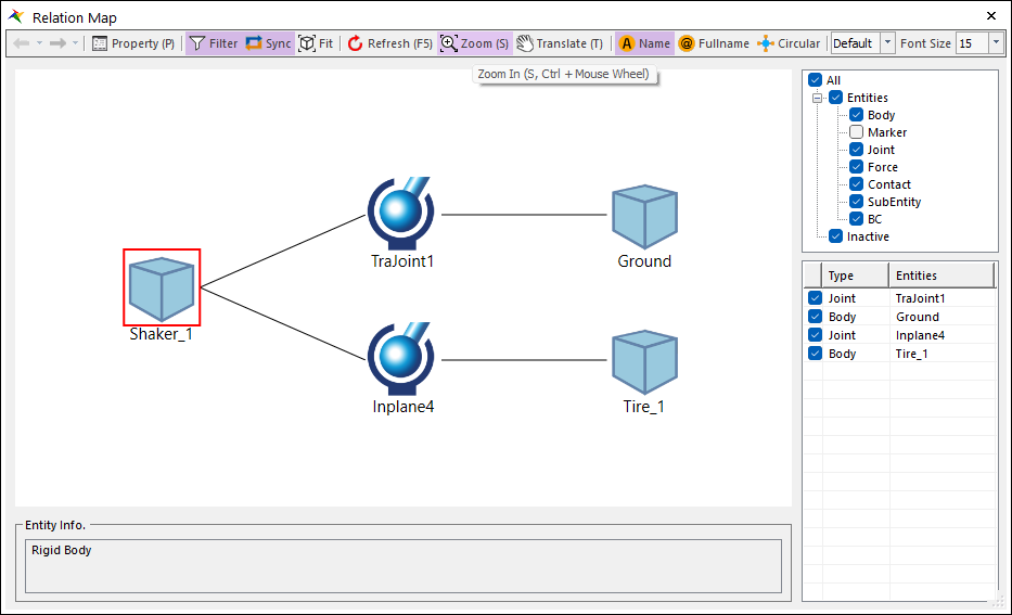
A shaker is prepared for each wheel of the vehicle. The shaker is connected to the ground with a translational joint so that it can only move up and down. It is also connected to the tire with an inplane joint so that it can only move in one surface. For further clarification, see the relational map provided with RecurDyn.

6.1.2.3.2. To save the model:

• In the File menu, click the Save As function.

  (You cannot perform the simulation if the model is in the tutorial path, so you must save the model in a different path.)

6.1.3. Defining Signals

6.1.3.1. Task Objectives

To run TSG, you should define the signals to be generated, define sensors to check the simulated response and process the measurement data.

6.1.3.2. Estimated Time to Complete This Task

5 minutes

6.1.3.3. Defining Actuators

Define actuators as many as the number of signals to be generated. Each defined actuator will be applied when you define the motion of the joint entity or the component of the force entity into an expression. In this tutorial, 4 shakers, each under a tire, are defined as translational joints and the displacement motion is applied to them to drive each tire up and down.

6.1.3.3.1. To create actuators:

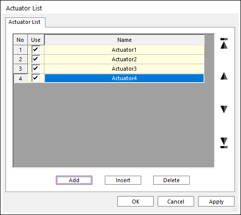
1. Click the Actuator Signal function in the TSG group under the Toolkit tab.

2. Define 4 actuators.

   

6.1.3.3.2. To apply actuators:

1. Click the Expression function in the Expression group under the Subentity tab.

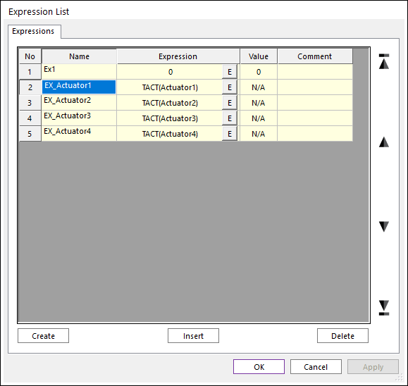
2. From the Expression List dialog window, click Create.

3. From the Expression dialog window, define the Name as EX_Actuator1 and enter TACT(Actuator1) in the Expression column.

4. Click OK to close the Expression dialog window. Also, for the remaining 3 actuators, create EX_Actuator2, EX_Actuator3 and EX_Actuator4.

   

5. Open the Properties dialog window for TraJoint1 and check the Include Motion option.

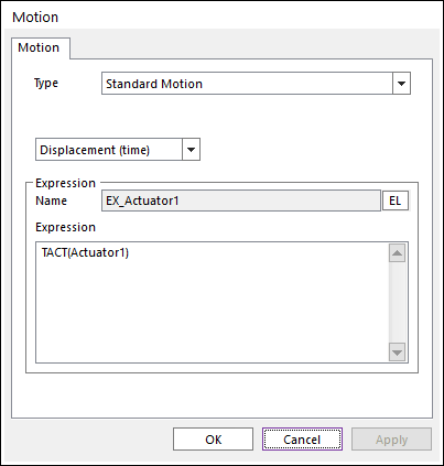
6. Click Motion to open the Motion dialog window.

   

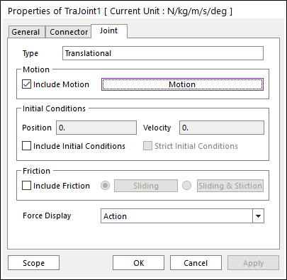
7. Set the Type field to Displacement (time) and click EL.

8. Import EX_Actuator1 created above from the Expression List dialog window.

   

9. Also, for TraJoint2, TraJoint3, and TraJoint4, fill the Motion dialog window for EX_Actuator2, EX_Actuator3, and EX_Actuator4 respectively.

6.1.3.4. Defining Sensors

The result derived from each sensor will be compared with the target signal as the performance index to check the simulated response. In this tutorial, the acceleration to the chassis will be measured.

6.1.3.4.1. To create sensors:

1. Click the Sensor Signal function in the TSG group under the Toolkit tab.

2. Click Add to open the Expression dialog window.

3. When the Expression dialog window appears, define it as follows:

   

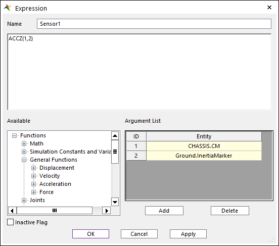
4. From the Expression dialog window, click OK.

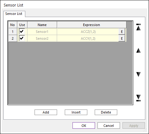
5. Make sure that it is added to the Sensor List dialog window.

6. Repeat the same steps above to create one more sensor ACCY(1,2). A total of 2 sensor signals should be created.

   

6.1.3.5. Defining Target Signals

These are the input data that you should define. They can be defined from a set of consecutive data over time obtained through test or simulation. These will be indices for TSG performance evaluation.

It is necessary to define Target Signals as many as the number of selected sensors. Target signals should be defined in the .csv file type in the order of time1, data1, time2, data2, ….

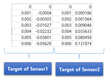
Consecutive data over time obtained from the test contain not only low frequency components but also a lot of high frequency components, which will cause noise and errors during the process of applying the TSG Toolkit. Therefore, it is recommended to use a low pass filter to include signals not greater than 50 to 100 Hz in the .csv file before creating it.

Since 2 sensors are defined in this tutorial, the .csv file should contain 4 sets of data created sequentially.

6.1.3.5.1. To create target signals:

1. Click the Target Signal function in the TSG group under the Toolkit tab.

2. From the Target Output List dialog window, go to the Target Output Function page and perform as follows:

   • Click … at the Target Signal field.

   • Select the ACCZ_ACCY_50hz_2EA.csv file located under the path where the initial model is.

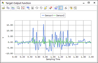
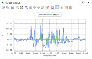
   • Check all fields in the Plot column and click Plot to view the target signal using a graph.

     

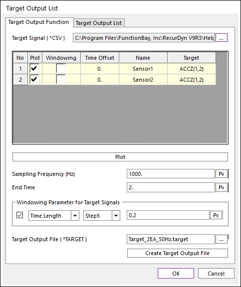
   • Enter 1000 in the Sampling Frequency field.

   • Enter 2 in the End Time field. The created .csv file contains 1000 pieces of data per second. You should consider this fact when you enter the end time.

   • Select Time Length for Windowing Parameter for Target Signals and enter 0.2 in the input field. And select Step5 Type for Windowing Method Type. This performs the function to forcefully set the start and end signals to zero to minimize errors when converting time signals to frequency signals through Fourier transformation.

   • Enter Target_2EA_50Hz.target in the Target Output File field to create a target file with the same name under the folder where the model is.

   • Click Create Target Output File.

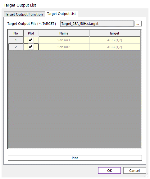
3. From the Target Output List dialog window, go to the Target Output List page and check the target signal created.

   • Check all fields in the Plot column and click Plot to view the target signal using a graph.

     

6.1.4. Performing FRF

6.1.4.1. Task Objectives

FRF (Frequency Response Function) derives a transfer function (H(f)), which represents system characteristics, through the signal processing course that converts the time signal to the frequency signal.

6.1.4.2. Estimated Time to Complete This Task

10 minutes

6.1.4.3. Performing FRF

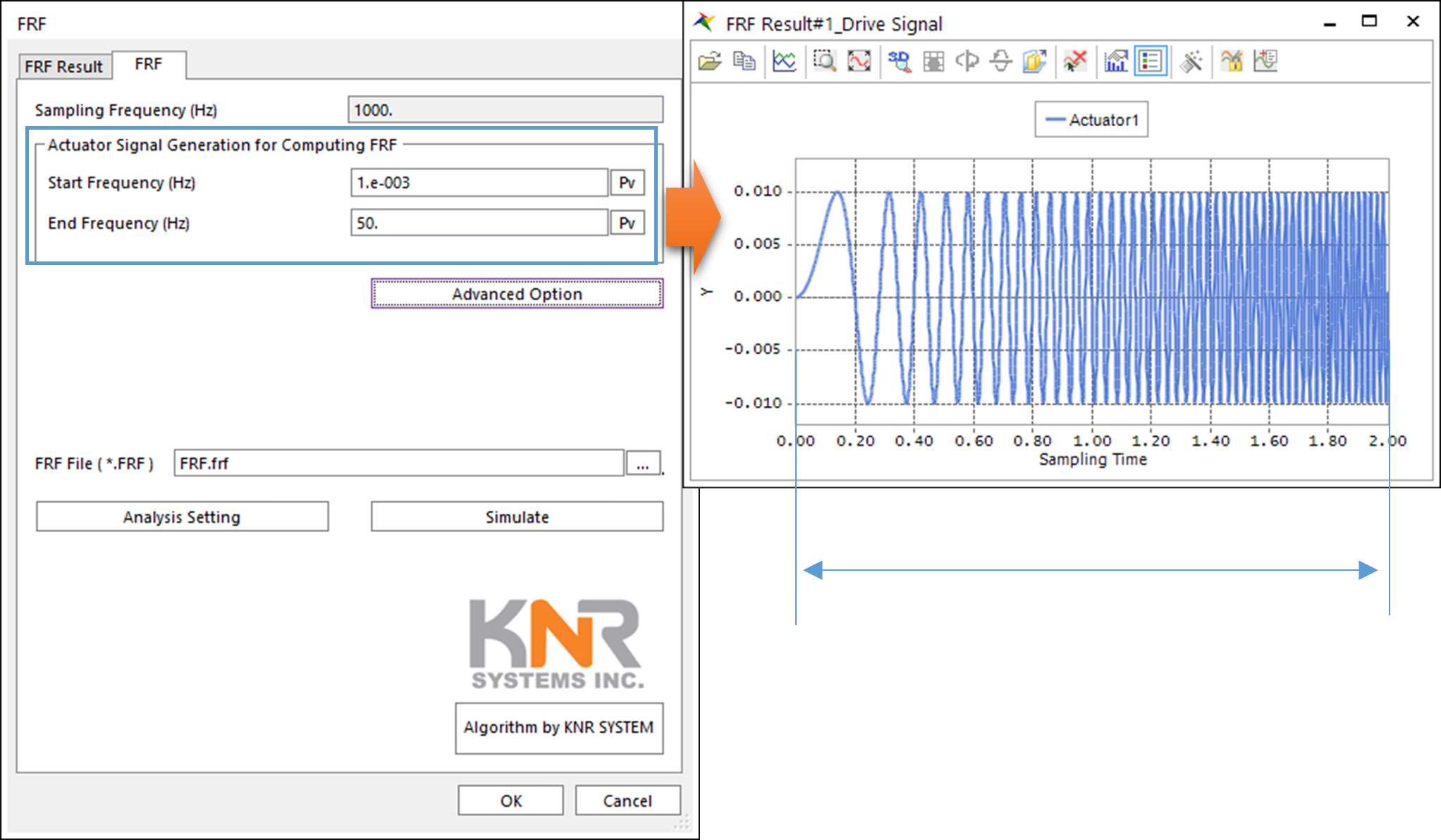
To perform FRF, the sweep sine function, which sequentially changes the input signal frequency, is applied to the parts to which expressions such as TACT(Actuator1) and TACT(Actuator2) are defined. The frequency band required at this moment is defined in the Start and End Frequency (Hz) fields.

1. Click the FRF function in the TSG group under the Toolkit tab.

2. From the FRF dialog window, perform as follows:

   • Enter 0.001 in the Start Frequency field.

   • Enter 50 in the End Frequency field. The target signal is filtered to 50 Hz or less. So, 50 Hz is applied to the End Frequency.

     

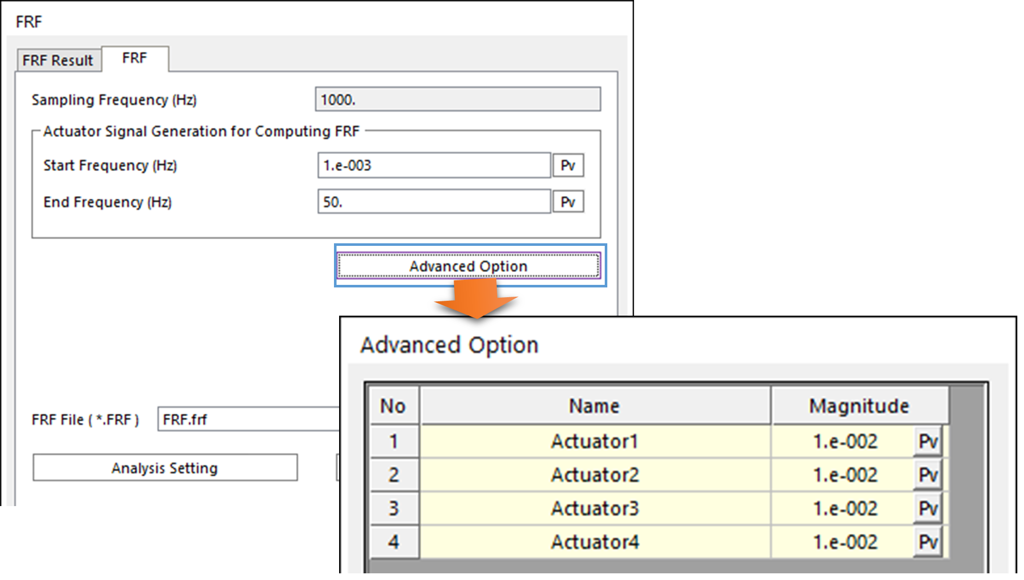
   • Click Advanced Option and enter 0.01 in the Magnitude field of the sweep sine function. In this tutorial, the model used the MKS unit. If the default setting, 1, is applied, the tire displacement changes in the unit of 1.0 m, which is an excessive condition.

     

   • Enter FRF.frf in the FRF File field to create a file with the same name under the folder where the model is.

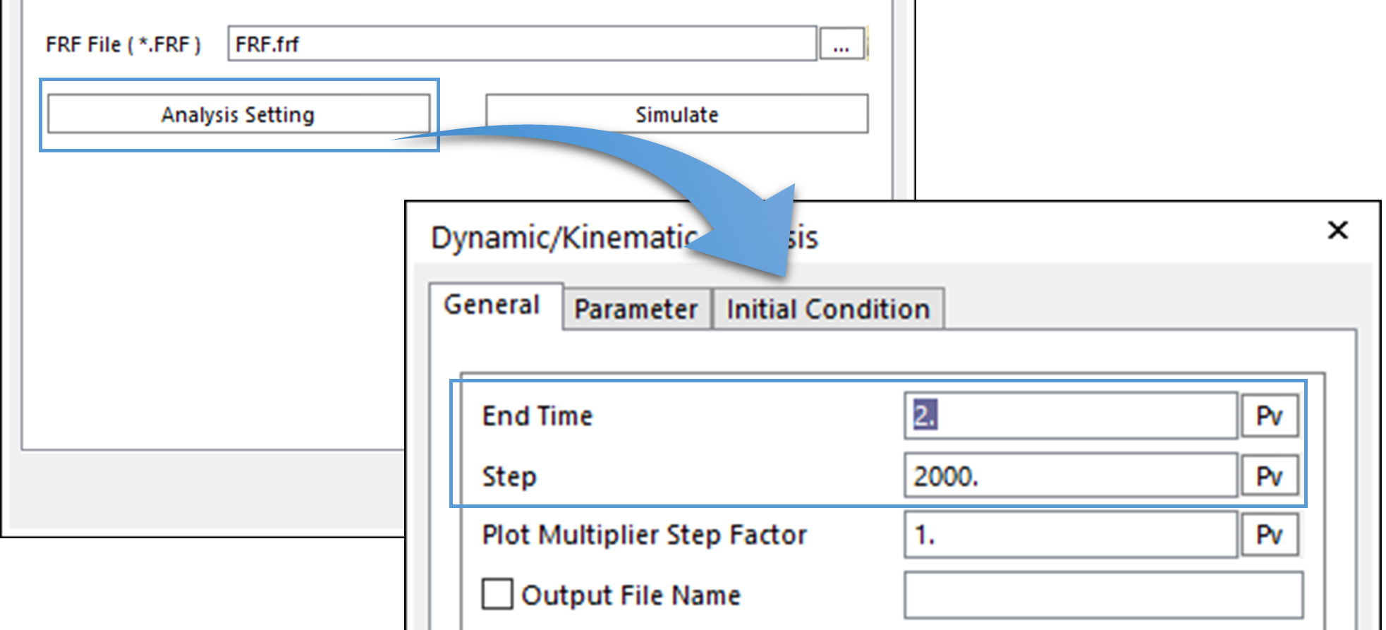
   • Click Analysis Setting and enter 2 in the End Time field and 2000 in the Step field. Importantly, the end time and the step should be set considering the sampling frequency when creating the target signal. In this tutorial, the sampling frequency is 1000 Hz. So, set the End Time field to 2 and the Step field to 2000.

     

   • Click Simulate to start the analysis. Analysis is performed as many times as the number of actuators configured.

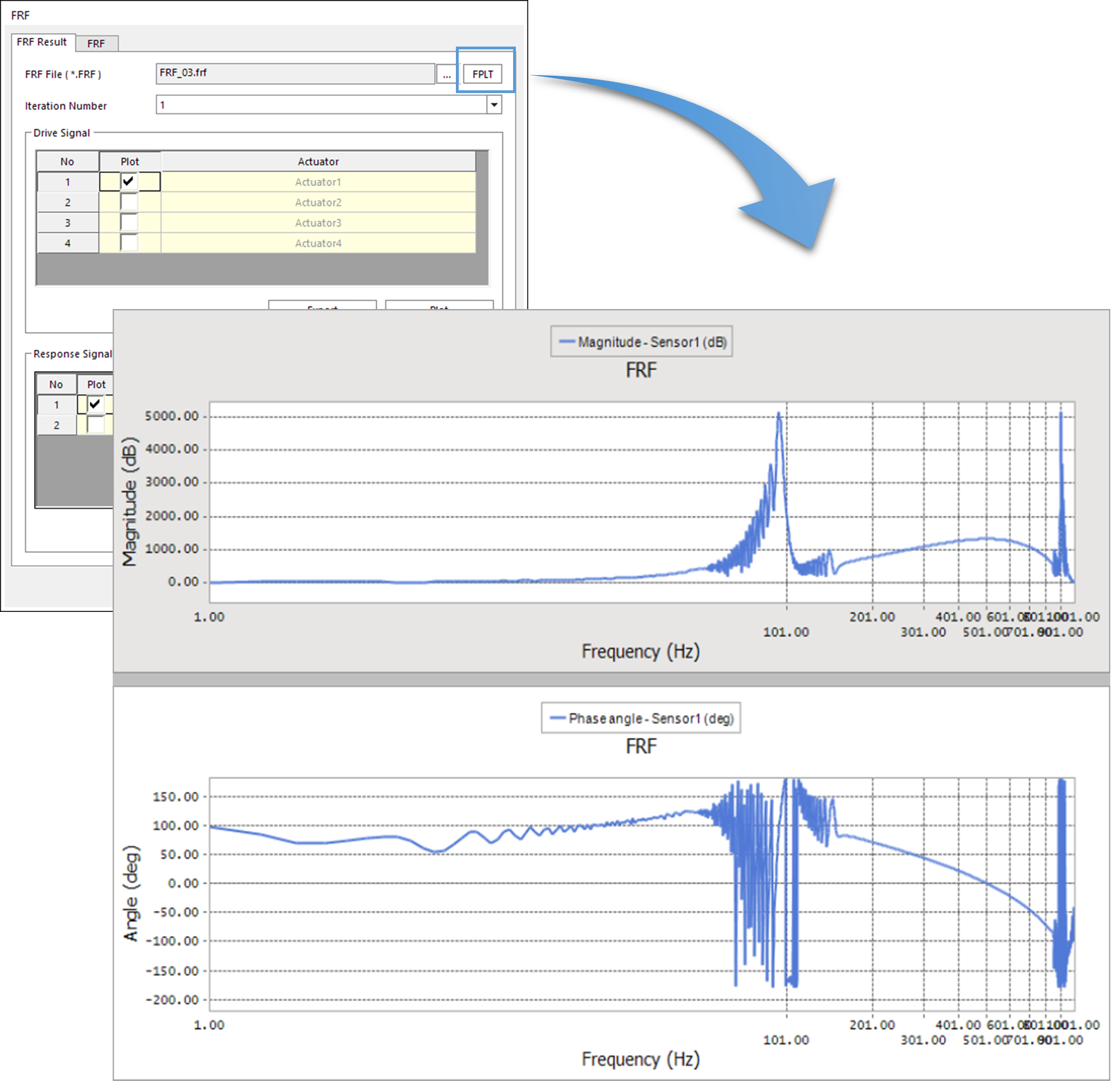
6.1.4.4. Viewing FRF Result

After performing FRF, you can view the result of the created frf file using a graph.

1. When the FRF analysis is completed, you will be moved from the FRF dialog window to the FRF Result page automatically.

2. Click FPLT to view the FRF result on the Plot Window.

3. Double-click the value you want to check in the Database of Plot.

   

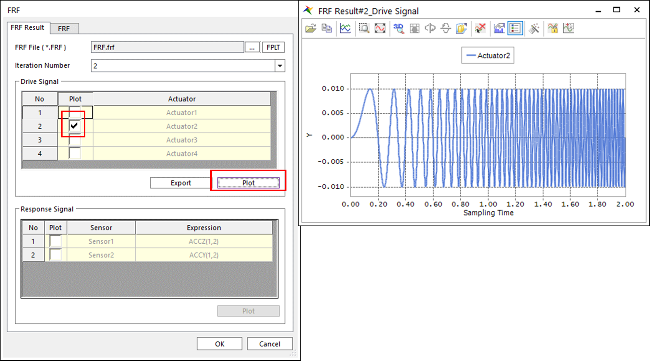
4. Click the FRF function again to open the FRF dialog window.

5. Set the Iteration Number field to 2, check the Plot option of Actuator2 in the Drive Signal table and click Plot to draw the drive signal for Actuator2 using a graph. The sweep sine function is applied to actuators individually in the FRF course. When an actuator is actuated, zero value is entered to the rest of actuators.

   

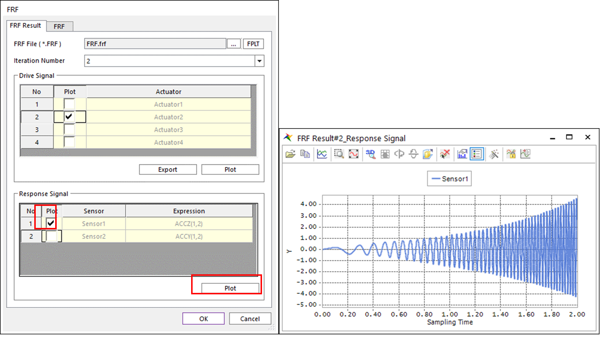
6. Check the Plot option of Sensor1 in the Response Signal table and click Plot to check it. The graph displays the result derived from the sensor when the sweep sine function is entered in the Drive Signal table.

   

6.1.5. Performing Iteration

6.1.5.1. Task Objectives

The Iteration course derives the drive signal applied to the actuator through iterative simulation to match the response signal measured from the sensor with the target signal defined by the user as much as possible based on the calculated FRF result.

6.1.5.2. Estimated Time to Complete This Task

10 minutes

6.1.5.3. Performing Iteration

Perform the analysis according to the following diagram.

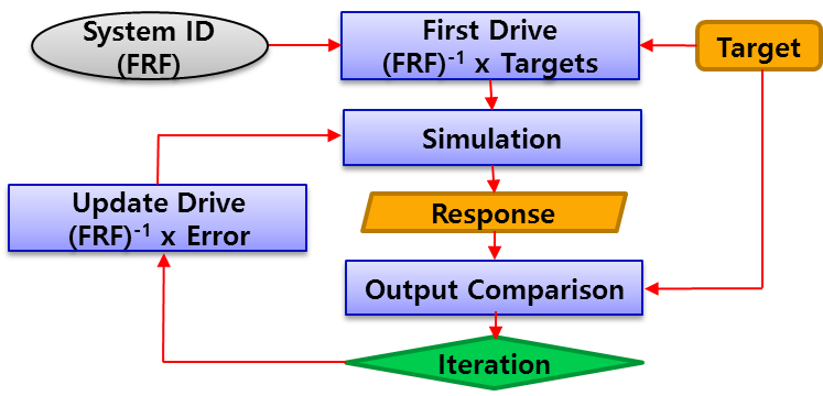
1. Click the Iteration function in the TSG group under the Toolkit tab.

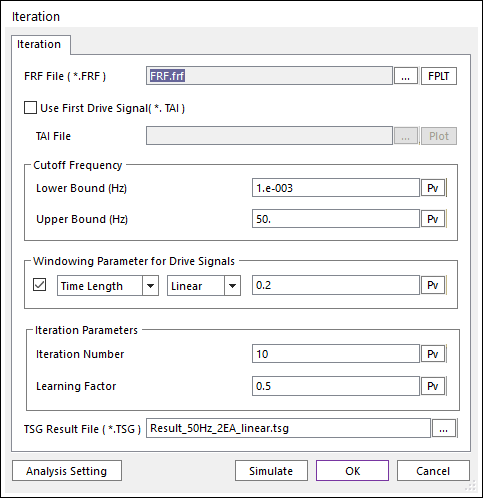
2. From the Iteration dialog window, enter data as follows:

   • Import the previously created FRF file by specifying the file name in the FRF File field. In general, the field is automatically filled.

   • For Cutoff Frequency and Windowing Parameter, use settings applied to the Target Output List dialog window and the FRF dialog window as is.

   • Enter 10 in the Iteration Number field to define the number of simulation iterations.

   • Enter 0.5 in the Learning Factor field to define the coefficient to compensate for the deviation between the target signal and the response signal.

   • Enter Result_50Hz_2EA.tsg in the TSG Result File field to create a result file with the same name under the folder where the model is.

     

   • Click Simulate to start the analysis.

6.1.5.4. Viewing Iteration Result

After performing the iteration course, you can view the result of the created tsg file using a graph.

1. When the iteration is finished, the Result dialog window appears automatically. (If you want to manually open it, click the Result function in the TSG group under the Toolkit tab.)

2. From the Result dialog window, perform as follows:

   • Select RMS for the Error Rate field and click the Plot button. The deviation between the target signal and the response signal is calculated using the RMS method each time iteration is performed, and the calculation result is displayed using a graph.

     

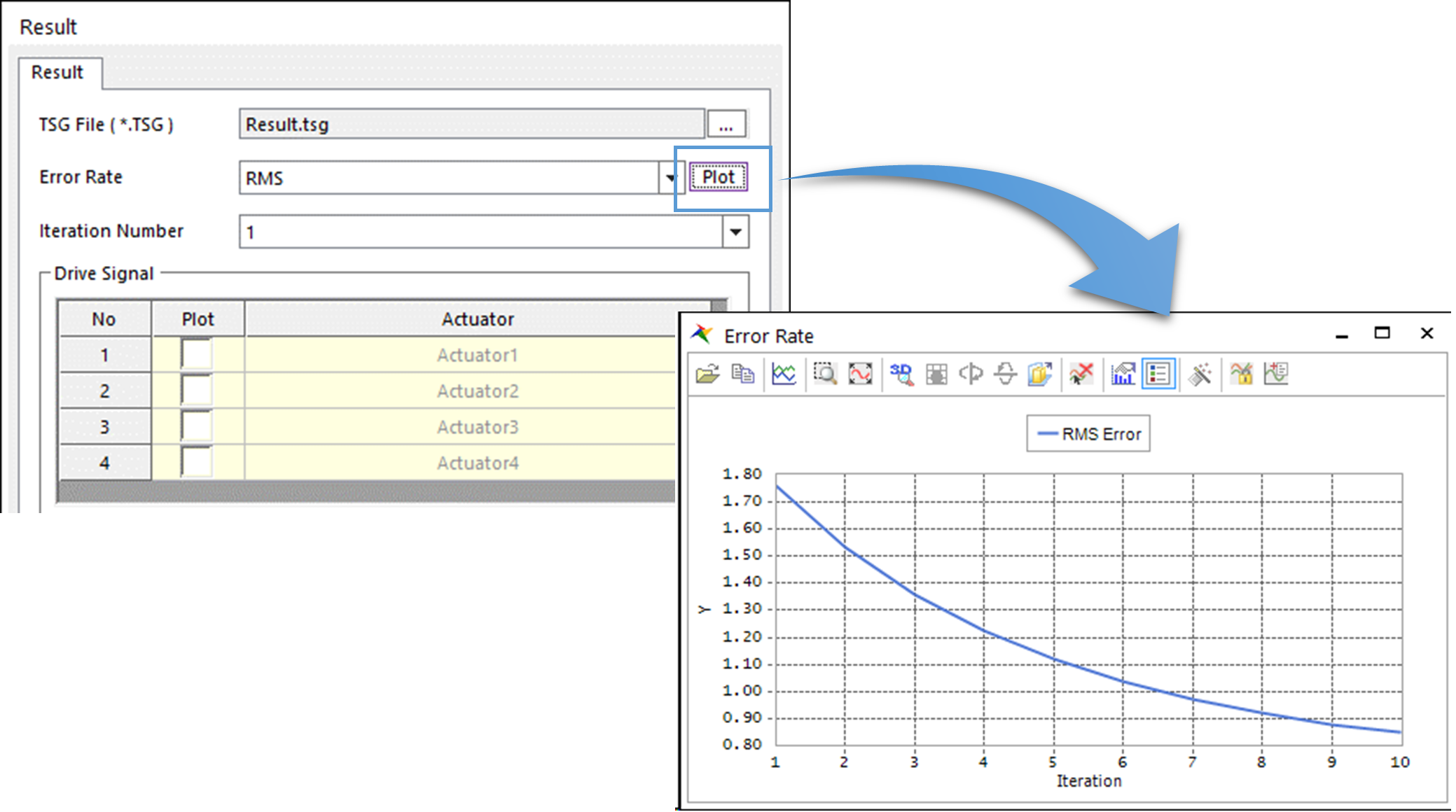
   • In the final analysis, the deviation rate becomes 0.85 approximately, which is the smallest value.

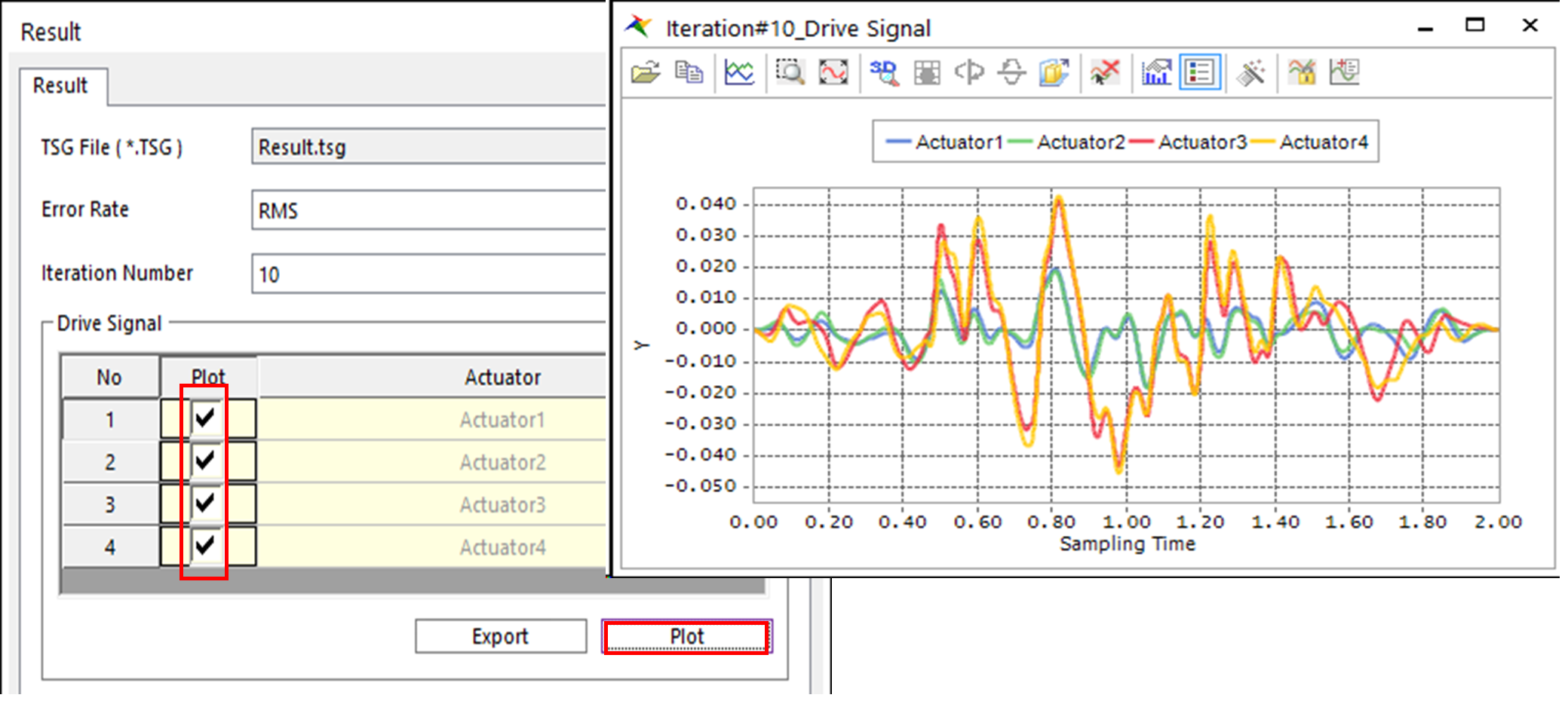
   • Set the Iteration Number field to 10, check all fields in the Plot column and click Plot to view the Drive Signal for all the actuators.

     

   • Set the Iteration Number field to 10, check the field for Sensor1 in the Plot column and click the Plot button to view the response signal for Sensor1 along with the target signal.

     

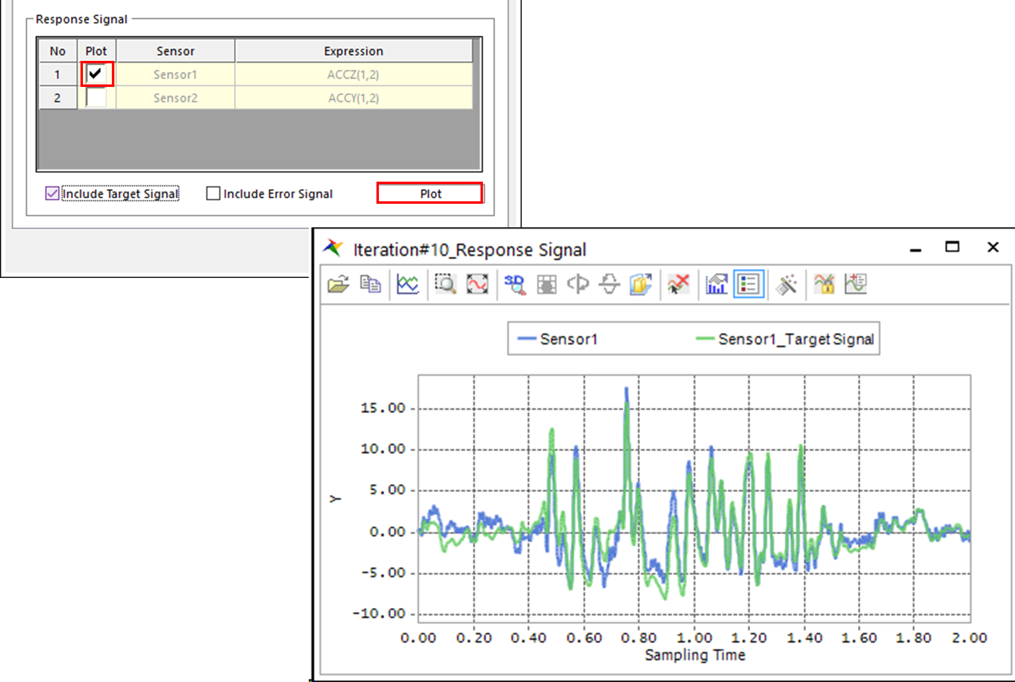
   • You can see that the Response Signal shows almost the same trend as the Target Signal. This means that there is no problem on the created Drive Signal.

3. From the Plot Window, export TSG/TimeSignalGeneration1/TSG Actuator values to a file to apply the values to other systems.