3.1. Three-Ball Contact Tutorial (AutoDesign)
3.1.1. Outline of Tutorial Sample A
Model |
Description |
Sample A |
Three-Ball Contact Problem: This problem explains the design process from making analysis model to formulating design optimization problem. This sample can help the beginners to understand a design optimization process in the AutoDesign. Key Point: Study the design formulation for representing contact phenomenon from the viewpoint of optimization. |
3.1.2. Three-Ball Contact Problem
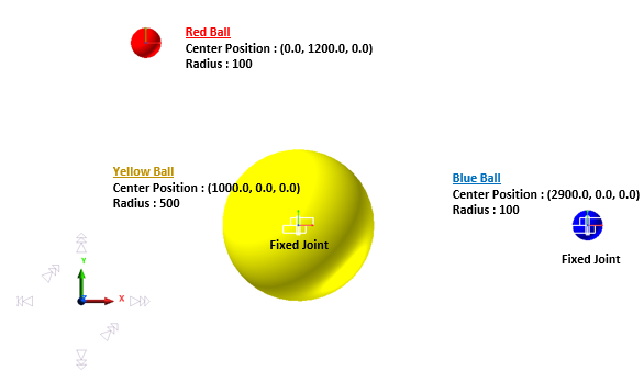
To explain the basic function of AutoDesign, let’s solve a simple design problem. The design model consists of three balls. The yellow and the blue ball are fixed on ground. When the red ball is thrown with an initial velocity, the red ball should be contacted with the yellow ball and go through the blue ball as near as possible.
Model Definition
Design Parameter Definition
Analysis Response Definition
Design Study
Design Optimization
Next, the refined optimization is explained to find more accurate results. This design uses the simulation results to solve the former design problem.
Refining the Design Formulation
Open files related in Sample-A |
|
Sample |
<InstallDir>\Help\Tutorial\AutoDesign\ThreeBallContact\Examples\Sample_A.rdyn |
Solution |
<InstallDir>\Help\Tutorial\AutoDesign\ThreeBallContact\Solutions\Sample_A.rdyn |
Note
If you change the file path at discretion, it can be located in any folder that you specify.
3.1.3. Model Definition
The contact between the red ball and the yellow ball is defined but is not done between the red ball and blue ball, because the blue ball is just the target point. The design variables are the initial velocity of red ball along x-direction and the contact stiffness coefficient in the contact force between the red and the yellow balls. Now, for the red ball to pass the nearest way to the center of the blue ball, what can you define as the design objective and constraints?
To do this, the design system is modeled as follows:
Figure 3.1 MBD Model of the ball contact design problem
The below is the procedure for defining the balls, joint and contact force shown in Figure 3.1.
Make balls shown in Figure 3.1 using the Ellipsoid function in the body module folder.
Fixed the Yellow ball and the Blue ball with ground using the Fixed joint in the joint module folder.
Define the contact force between the red ball and the yellow ball using the Sphere To Sphere contact in the contact module folder.
3.1.4. Design Parameter Definition
Let’s study the procedure for defining design parameters:
Define parametric values shown in Figure 3.2.
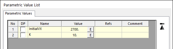
Figure 3.2 Parametric value definition
Link the InitialVX with the x direction initial velocity of the red ball body shown in Figure 3.3.
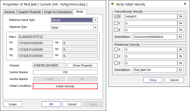
Figure 3.3 Link the InitialVX
Link the K with the stiffness coefficient of the contact force between the red ball and the yellow ball shown in Figure 3.4.
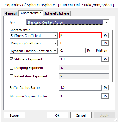
Figure 3.4 Link the stiffness K
Define the design parameters from parametric values using the Design Parameter command in the AutoDesign toolkit shown in Figure 3.5 and Figure 3.6. First, you push Create button to define the design parameters as Figure 3.5. In Figure 3.6, you should link the design parameters to the parametric values that were defined in Figure 3.2. The initial values are the current parametric values defined in Figure 3.2. You should define the lower and the upper bounds on the design variable. This represents that the optimization process should change the design values within these bounds during iterations. After you create the design parameters, you check the active design parameters for this design problem.
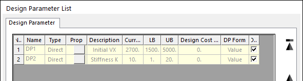
Figure 3.5 Check DV check box
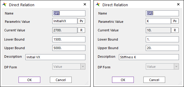
Figure 3.6 Define DP1 and DP2
3.1.5. Analysis Response Definition
The design goal is that the center of the red ball passes the nearest way from the center of the blue ball, the target point. You need to define the performance indexes for solving the optimization problem. In AutoDesign, performance indexes are objectives and constraints in design optimization, which are composed of analysis responses. Then, in order to define the performance index, analysis responses are defined first. The procedure of defining analysis responses is explained as:
Define Expressions shown in Figure 3.7. Each expression is defined shown in the Figure 3.8, Figure 3.9, and Figure 3.10, sequentially.
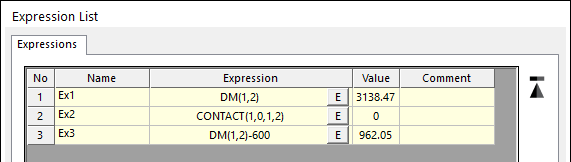
Figure 3.7 Expression List
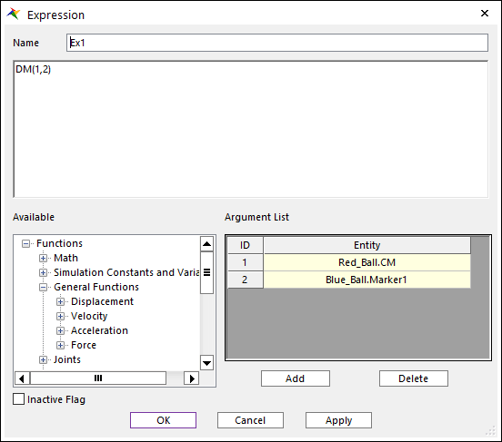
Figure 3.8 Detailed Definition of Expression Ex1

Figure 3.9 Detailed Definition of Expression Ex2
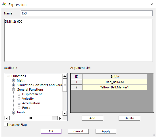
Figure 3.10 Detailed Definition of Expression Ex3
Register expressions for analysis response shown in Figure 3.11. Other figures are representing the dialogue of each analysis response. Define the Analysis Response using the Analysis Response command in the AutoDesign toolkit. The detailed information for each analysis response is shown in Figure 3.12. Also, their physical relations are shown in Figure 3.13.
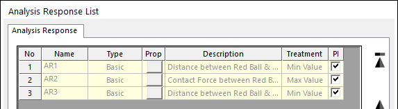
Figure 3.11 Analysis Response List
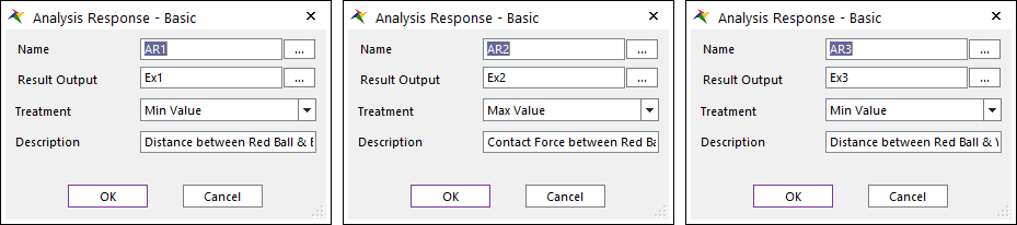
Figure 3.12 The detailed information for three analysis responses
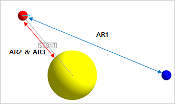
Figure 3.13 Three analysis responses in the model
3.1.6. Design Study
Before you start to solve this optimization problem, it needs to know the relationship between design variables and analysis responses or the correlation between analysis responses. To get that kind of information, you need the effect analysis from design of experiments. AutoDesign provides such functions as effect analysis, correlation analysis and even design variable screening in Design Study menu. Design Study is composed of six sub-menus listed in Table 3.1.
Design Variables |
Select DOE method and define the level for variable |
Performance Index |
Show the ARs checked in Analysis Response menu |
Simulation Control |
Define the solving option of RecurDyn solver |
Effect Analysis |
Perform the effect analysis from the analysis results |
Screening Variables |
Screening procedure from the effect analysis results |
CorrelationAnalysis |
Perform the correlation analysis from analysis results |
3.1.6.1. Basic Procedure for Design Study
In order to design study such as effect analysis, screening variables and correlation analysis, you select the DOE method and define the level for each variable and perform the simulation of RecurDyn. First, these procedures are explained as:
In the sub-menu of design variables, select Bose’s Orthogonal Design in DOE methods, and set the level of the study as 5. Then, one defines the required runs as 25. This method is a strength-II orthogonal array design. For more information, one may refer to the theoretical manual of AutoDesign.
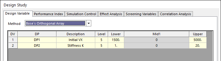
Figure 3.14 Define DOE method for design study
Confirm the Performance index that is checked in Analysis Responses.
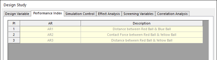
Figure 3.15 The selected PI list for design study
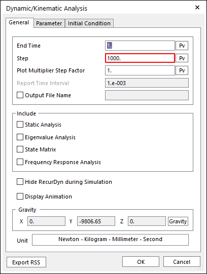
In the sub-menu of simulation control, define analysis setting shown in Figure 3.17 and Figure 3.18. This setting is the same as that in RecurDyn analysis. If you increase the accuracy of effect analysis and optimization results, it is recommended that the plot multiplier factor should be 1.0 and increase the number of steps. After setting the options, push OK. After setting them, push the Execution button. Then, RecurDyn is analyzed for the given number of trials.
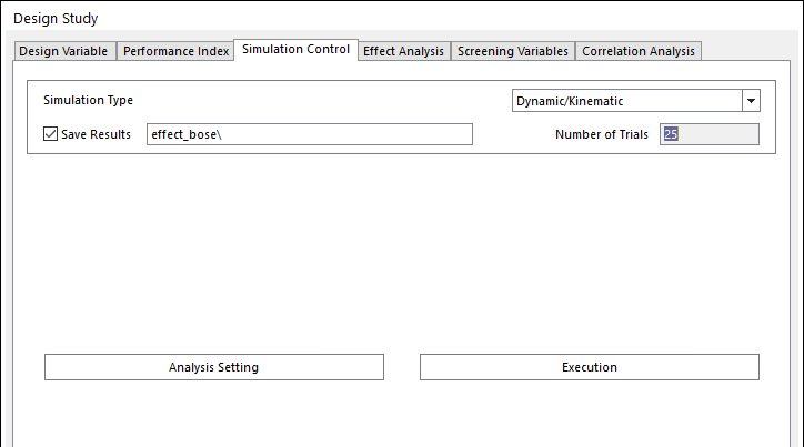
Figure 3.16 Simulation Control page
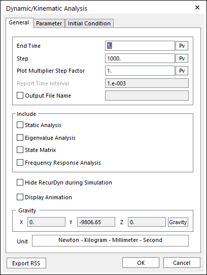
Figure 3.17 General analysis setting
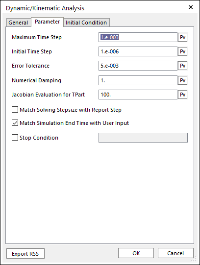
Figure 3.18 Integrator parameter setting
After all analyses are completed, one can select the effect analysis, correlation analysis and screening design variables.
Now, select the effect analysis menu. Effect analysis gives the relation between one performance index and all design variables.
3.1.6.2. Effect Analysis
Figure 3.19 shows the effect analysis menu. Let’s study the effect analysis procedure.
Select the performance index in PI row. Then check the design variables to see the effect analysis for the selected PI. Then, push Draw. Figure 3.20 shows the effect analysis between PI_1 and design variables. This shows that DV1 is more nonlinear than DV2 in the distance between red ball and blue ball.
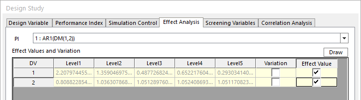
Figure 3.19 Sub-menu for effect analysis
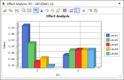
Figure 3.20 Effect analysis result for the first PI
Similarly, you can see the effect analysis for PI_2, which is shown in Figure 3.21. For the 4th and 5th levels of DV1, the contact forces are zero. This represents that two balls are not contacted for those cases. It is noted that this discontinuity makes the accuracy of meta-model to be worse.
Figure 3.21 Effect analysis result for the second PI
Finally, you can see the effect analysis for PI_3, which is shown in Figure 3.22. This represents the distance between red and yellow balls. Unlike Figure 3.21, this shows a continuous result even though two balls didn’t contact for 4th and 5th levels of DV1. This represents that PI_3 is suitable to define the contact constraint in the design optimization.
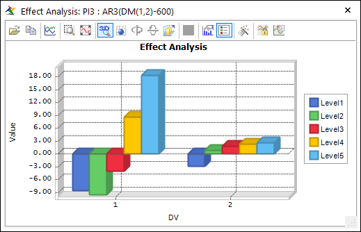
Figure 3.22 Effect analysis result for the third PI
The explanation of effect analysis is completed. However, you have a question for the minimization or maximization combinations shown in Figure 3.23.
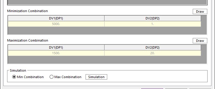
Figure 3.23 Selection of minimization or maximization combination
Suppose that you select the third PI. Then, you see the effect analysis result shown in Figure 3.22. Then, Figure 3.23 shows the design variable combination for minimizing PI_3 and maximizing PI_3. If you need the confirmation for minimum or maximum set, then select one of them and push simulation button in Figure 3.23 menu.
3.1.6.3. Screening Variables
Figure 3.24 shows the menu for screening variables. First, you can see the scatter points. This represents the design variables. In this problem, there are only two design variables. Thus, variable screening is not required but we study only the screening variable method.
First, select the first performance index, PI_1. Figure 3.24 shows that two design variables have severely different effectiveness. Now, you need to know which variable is effective for PI_1.
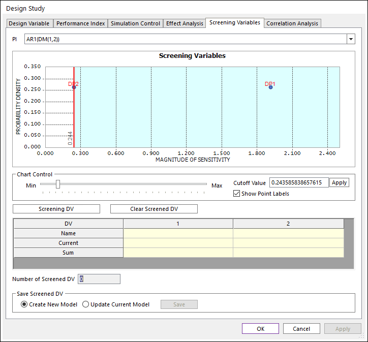
Figure 3.24 Sub-menu for screening variables
Define the cutoff values as 1.0 and push Apply. You can see Figure 3.25. Then, push Screening DV. Figure 3.26 shows the screening result. It shows that design variable DV1 (or DP1) is more effective than DV2.
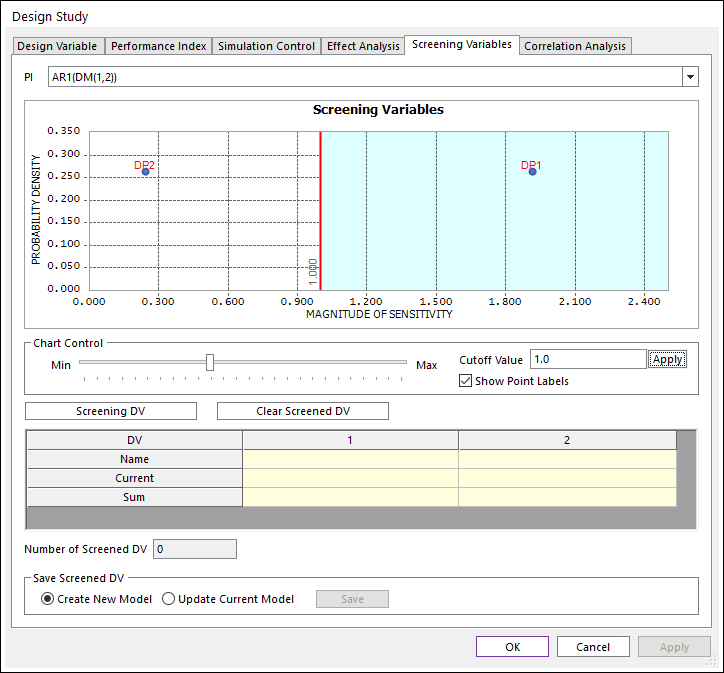
Figure 3.25 Defining the cutoff value for screening variables
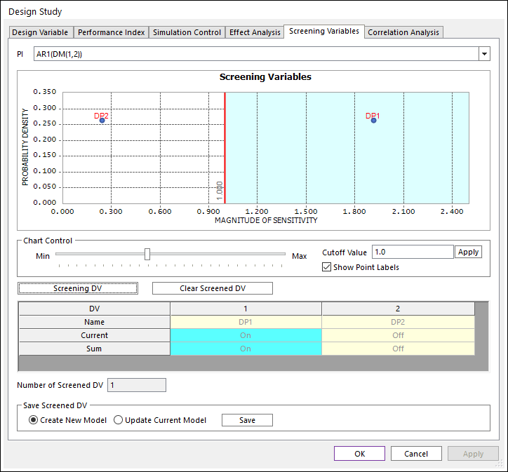
Figure 3.26 Screened result for the first performance index
Next, change the performance index AR3. Then, define the cutoff value as 12. Perform the similar procedure in step 2. Then you can see the result shown in Figure 3.27. In the figure, Current represents the screening results for PI_3. Total represents the union of screening results for PI_1 and PI_3. If you push Save button, only active design variables (marked ‘on’) are remained in New Model or Current Model.
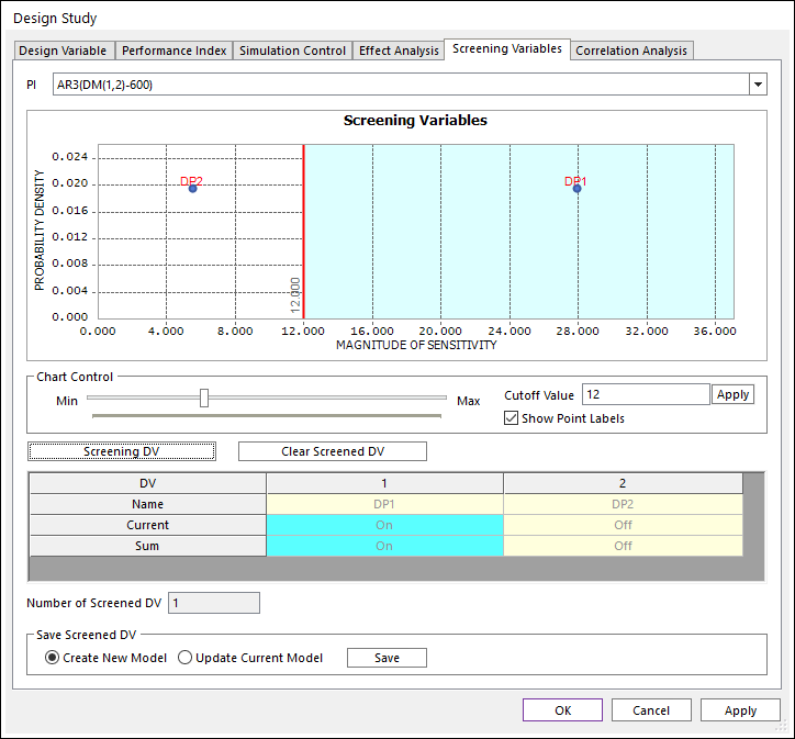
Figure 3.27 Screened result for the third performance index
3.1.6.4. Correlation Analysis
Figure 3.28 shows the menu for correlation analysis. This shows the relation between two selected ARs from the analysis results. If you see the relation between the first PI and the third PI, check Horizontal Axis as PI_1 and Vertical Axis as PI_3 and push Draw. Then, you can see the correlation result shown in Figure 3.29. Figure 3.29 shows that they have no trend or slightly reverse trend.
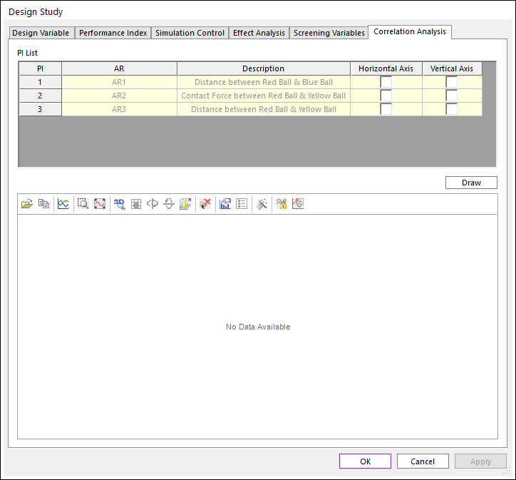
Figure 3.28 Sub-menu for correlation analysis
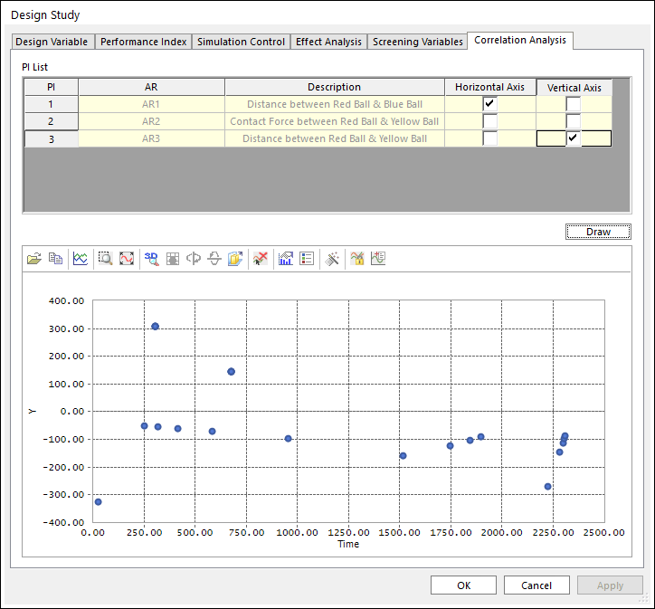
Figure 3.29 Correlation result between PI_1 and PI_3
3.1.7. Design Optimization
3.1.7.1. Let’s remind the following design problem:
Find the initial velocity of red ball along x-direction and the contact stiffness between red and yellow balls for red ball to hit the blue ball after red ball hit yellow ball.
Next process is for defining the design option and executing the optimization analysis. The first step is to define the design variables shown in the Figure 3.30. This can start using the Design Optimization command in the Auto Design toolkit.
In Design Variable menu, the selected DPs are listed. In this menu, DP can be design variable or constant during optimization process. If you define a DP as constant, you should define its constant value.
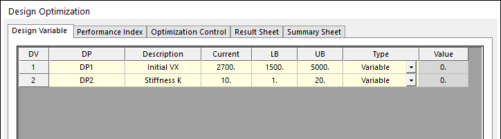
Figure 3.30 Definition of design variables
The next process is to define the performance indexes in Figure 3.31, which is named as performance index of the dialog of Figure 3.30. Performance Index is a design optimization formulation part. Figure 3.32 shows the mathematical definition for design optimization. Let’s discuss the optimization formulation in Figure 3.31. In the first performance index, choose AR1 and define it as objective. Also, select the design goal as minimization and define its weighting coefficient as 1.0. In the second performance index, add one inequality constraint as AR1 =< 100. In the third performance index, add one inequality constraint as AR3 =< 0, In the last performance index, choose AR2 and define it as objective. Unlike AR1, the design goal is defined as maximization and its weight coefficient is defined as 1.
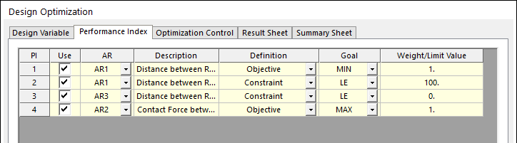
Figure 3.31 Definition of performance indexes
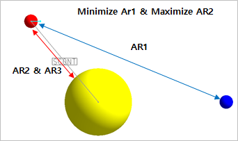
Figure 3.32 Design optimization formulation
Check the analysis setting by clicking Analysis Setting. In order to reduce the numerical error, we increase the number of time steps shown in below. If you increase the resolution of optimization solution, then increase the number of steps. In refining the design optimization, we will show more accurate design by only increasing the value.
Define the option of optimization control and execute analysis shown in the Figure 3.33. The analysis setting is the same that of Design Study. Finally, if you push the optimization button, you can see the summary of the design optimization formulation shown in Figure 3.34. Then, check your formulation. If you see some mistakes, then push Cancel and correct the mistakes. Otherwise, push the Execution button. Then, AutoDesign runs until convergence criteria are satisfied or maximum iteration is reached. During optimization process, you can see the analysis results in the Simulation History menu.
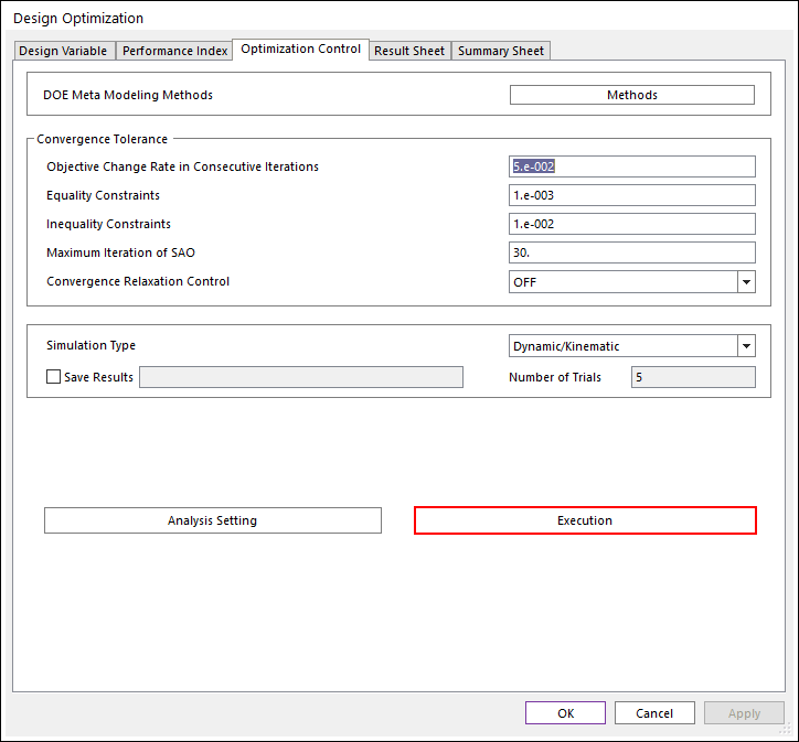
Figure 3.33 Control option definition for optimization and analysis
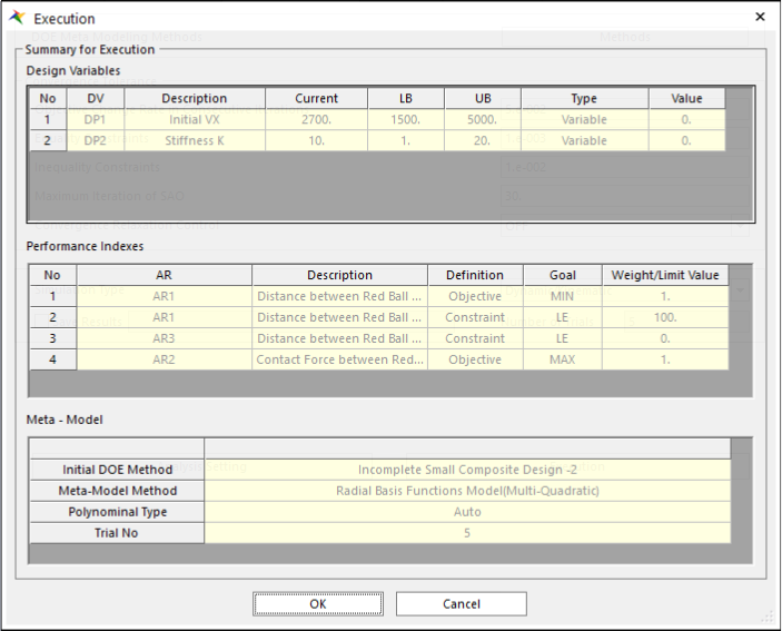
Figure 3.34 Summary of design optimization formulation
If AutoDesign is completed, then you can see the convergence results in Result Sheet. Figure 3.35 shows the optimization results. In RecurDyn, the final value of AR1 is 16.769(mm) after 15 iterations. Figure 3.36 shows the trajectory of red ball for SAO 10.
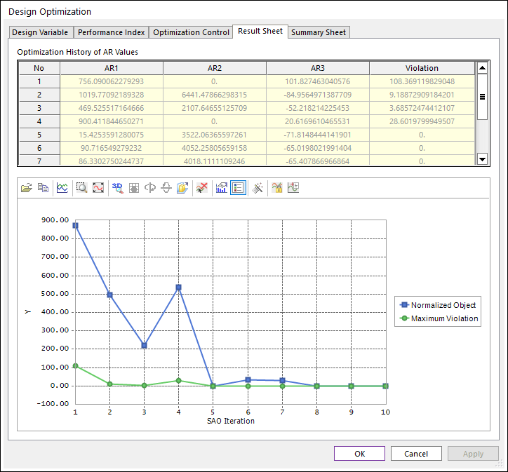
Figure 3.35 Convergence history
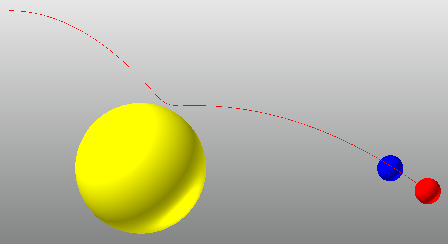
Figure 3.36 Animation of the final design