8.1. Vibrating Transmission (Acoustics)
8.1.1. Overview
As the quality of human life improves, many efforts are being made to control noise and vibration in various industries. In the mechanical industry, it is very important to find out the part that generates a large amount of vibration and the frequency band with a large amplitude.
The example model used in this tutorial is a link system that makes rotary motion into the reciprocating motion with a vibrating transmission. When analyzing the vibration generated in the housing of this mechanical system, it is difficult to analyze clearly where and what kind of vibration occurs from the result of the existing FE analysis alone.
Therefore, this tutorial introduces and explains a method to calculate the ERP (equivalent radiated power) generated in the housing by using the post tool called Acoustics, which analyzes the noise vibration, and a method of analyzing the vibration occurring in the housing using the post functions.
8.1.1.1. Task Objectives
This tutorial covers the following topics:
How to replace RFlex Body through RecurDyn/RFLEX
How to perform ERP calculation and analysis through RecurDyn/Acoustics
8.1.1.2. Prerequisites
This tutorial is intended for users who have completed the Basic and FFlex/RFlex tutorials provided with RecurDyn. If you have not completed these tutorials, then you should complete them before proceeding with this tutorial. In addition, this tutorial requires a basic understanding of dynamics and the finite element method.
8.1.1.3. Procedures
The following table outlines the tasks involved in this tutorial and their duration.
Procedures |
Time (minutes) |
Simulating and analyzing the initial model |
5 |
Changing an existing body to the RFlex body |
15 |
Calculating equivalent radiated power |
15 |
Modifying and analyzing the model |
15 |
Total |
50 |
8.1.1.4. Estimated Time to Complete this Task
75 minutes
8.1.2. Simulating and analyzing the initial model
8.1.2.1. Task Objectives
Open the initial model, perform a simulation, and observe the behavior of the vibrating transmission.
8.1.2.2. Estimated Time to Complete This Task
5 minutes
8.1.2.3. Opening the Model
8.1.2.3.1. To copy the example model:
Copy the Acoustics tutorial example folder provided by RecurDyn to an analyzable location.
Folder path: <InstallDir>\Help\Tutorial\PostAnalysis\Acoustics\VibratingTransmission
8.1.2.3.2. To run RecurDyn and open the initial model:
On the Desktop, double-click the RecurDyn icon to run RecurDyn. The Start RecurDyn dialog window will appear.
When the Start RecurDyn dialog window appears, close it.
In the File menu, click the Open function.
In the Acoustics folder copied above, select VibratingTransmission_Start.rdyn.
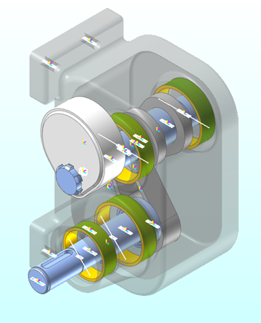
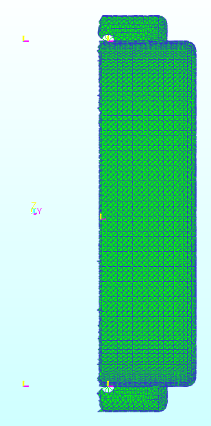
Click Open. The model appears as shown in the following figure.
8.1.2.3.3. To analyze the model:
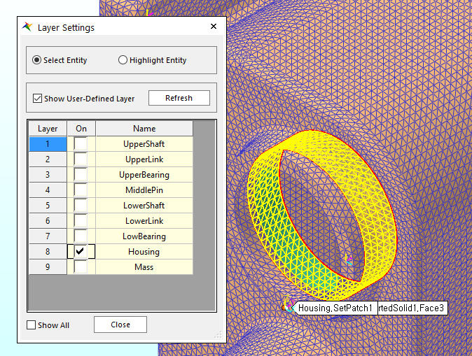
Click the Layer Settings tool in the Render Toolbar.
In the Layer Settings dialog window, turn on and off each layer to analyze the model.
The following explains the configuration of the model.
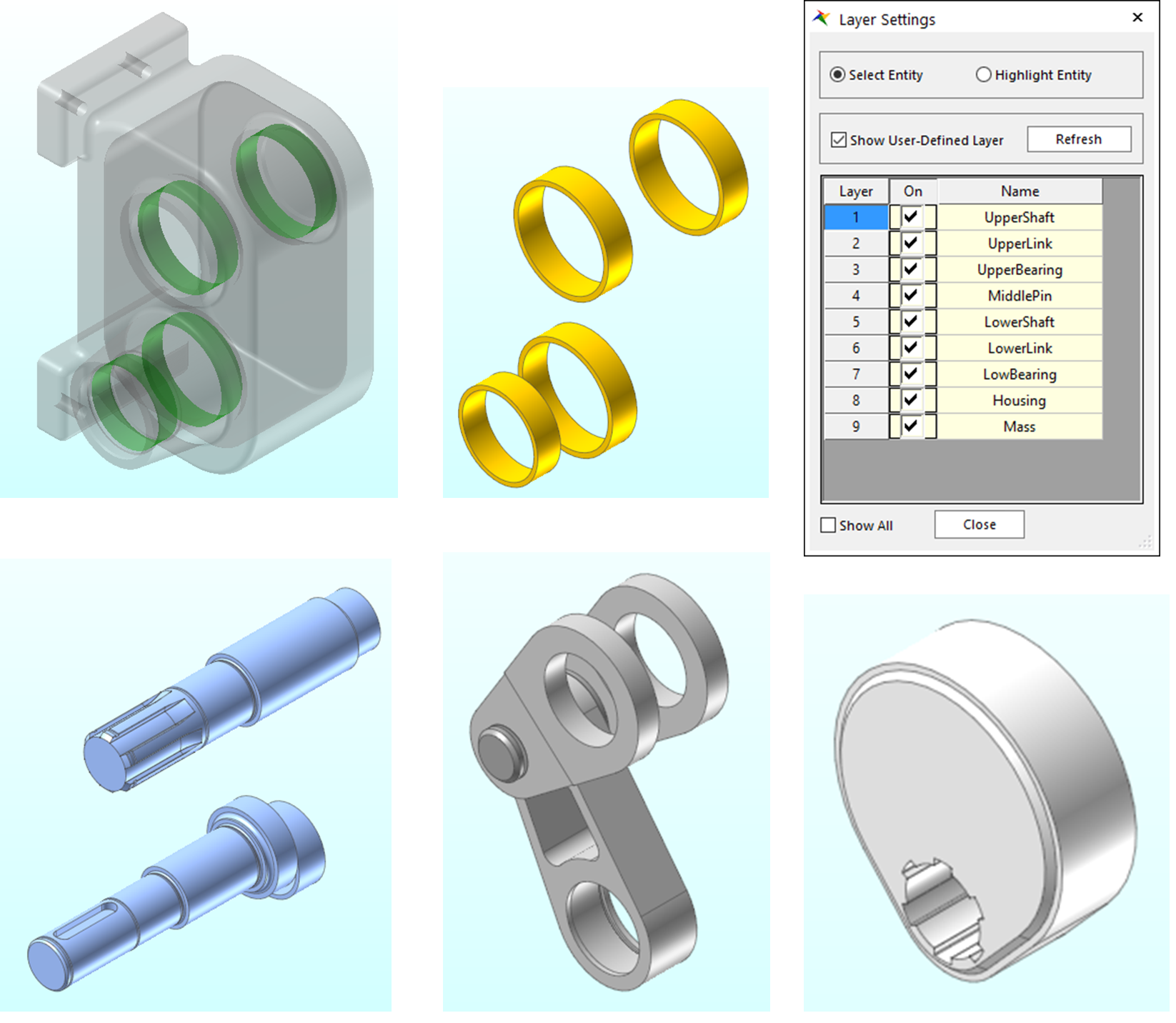
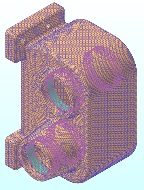
The Model generally consists of 5 parts: Housing, Bearing, Shaft, Link, and Mass. When the rotary motion is delivered from the lower drive shaft, the pendulum on the upper shaft performs the periodic motion through the link system.
The connection between the shaft, bearing and link are all made up of bushing force, and the housing and bearing are composed of GeoSurContact.
The drive shaft is driven by CMotionGroup and rotates at 100 * 2PI per second.
8.1.2.4. Performing Simulation
Run the simulation to help you understand the model system.
8.1.2.4.1. To run the simulation:
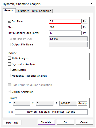
On the Analysis tab, in the Simulation Type group, click the Dynamic / Kinematic Analysis function. The Dynamic/Kinematic Analysis dialog window appears.
After verifying the simulation conditions, click Simulate.
End Time: 0.1
Step: 500
8.1.2.4.2. To view the result:
Under the Analysis tab, in the Animation Control group, press the Play function to check if the system operates as shown in the figure below.
As described in the Analyzing the model section, the motion delivered from the lower drive shaft is transmitted to the link system, and finally the mass on the upper shaft makes a periodic motion.
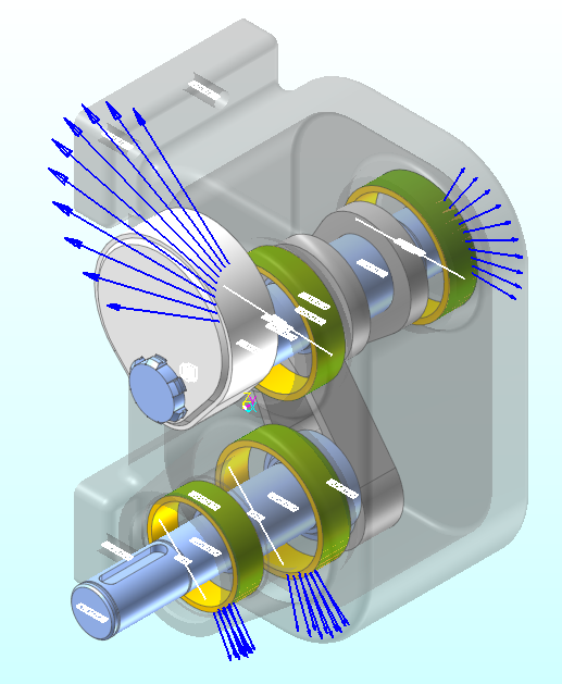
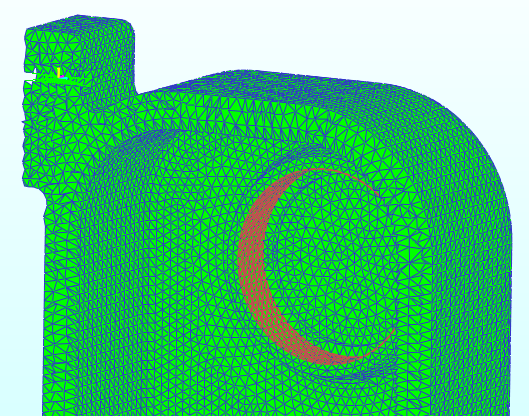
In the process of power transmission as shown in the figure, the housing receives contact force from 4 bearings.
If you observe the force display of the contact force, you can notice that it moves at a certain cycle. To analyze how this external force directly affects the housing, it is necessary to change the housing, which is a rigid body, to a flexible body.
8.1.3. Changing an existing body to the RFlex body
Since the housing of the RecurDyn model is a rigid body, you cannot see the deformation of the body due to external force. Therefore, we will perform the RFlex Body Swap function provided by RecurDyn to replace the housing with a flexible body. In addition, the Acoustics Post Tool to be performed in the later chapter can only be performed on a flexible body.
8.1.3.1. Task Objectives
In this chapter, you will learn how to change an existing rigid body to a flexible body using the RFlex Body Swap function provided by RecurDyn/RFlex.
8.1.3.2. Estimated Time to Complete This Task
15 minutes
8.1.3.3. Modifying a Model Using a RFlex Body
8.1.3.3.1. To swap with a RFlex Body:
On the Flexible tab, in the RFlex group, click the Import RFI function.
Change the modeling option to Body.
In the Working Window, select the Housing using the mouse as shown below. The RFlex Body Import dialog window appears.
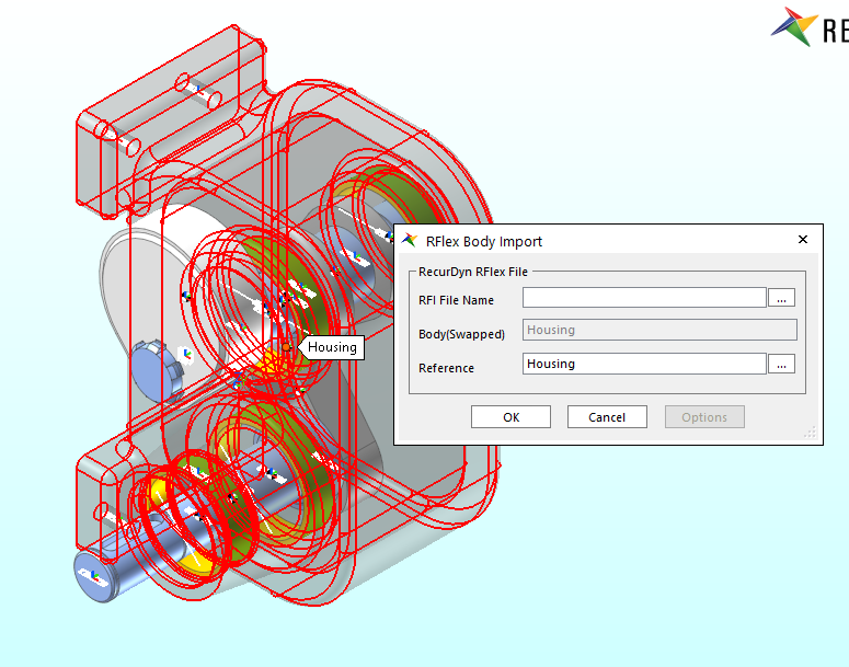
In the RFlex Body Import dialog window, perform the following:
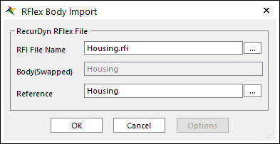
Press … button in the RFI File Name field.
Select the Housing.rfi file located in the Acoustics folder copied in Chapter 2.
Verify that the selected conditions match those shown in the figure to the below, and then click OK.
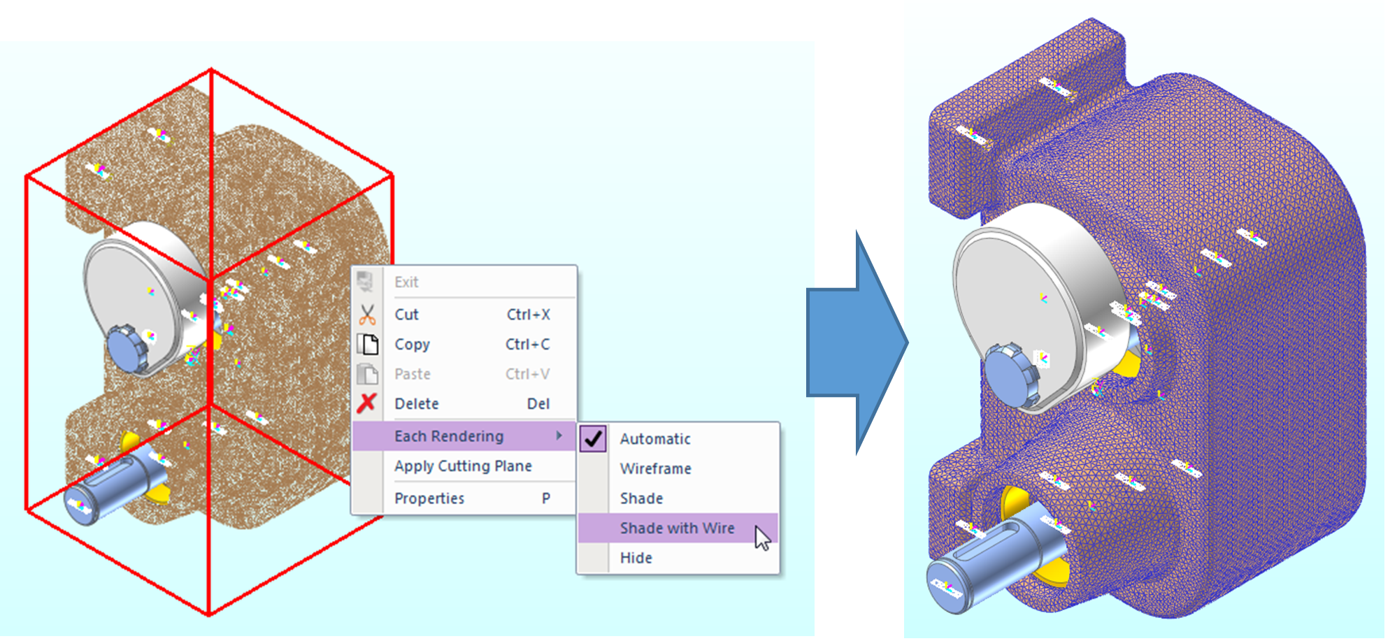
You can verify that the housing was replaced by a RFlex body.
The swapped housing looks like a wire frame. Change each rendering just like the previous housing.
8.1.3.3.2. To change each rendering:
In Working Window, select the housing that changed to a RFlex body.
Right-click the Working Window.
In the pop-up menu, change Each Rendering to Shade with Wire.
8.1.3.4. Redefining Contact
When changing from a rigid body to a RFlex body, the information about contact patches will disappear and all existing GeoSurContact will also disappear. After creating the patches again in the housing, you need to redefine the contact.
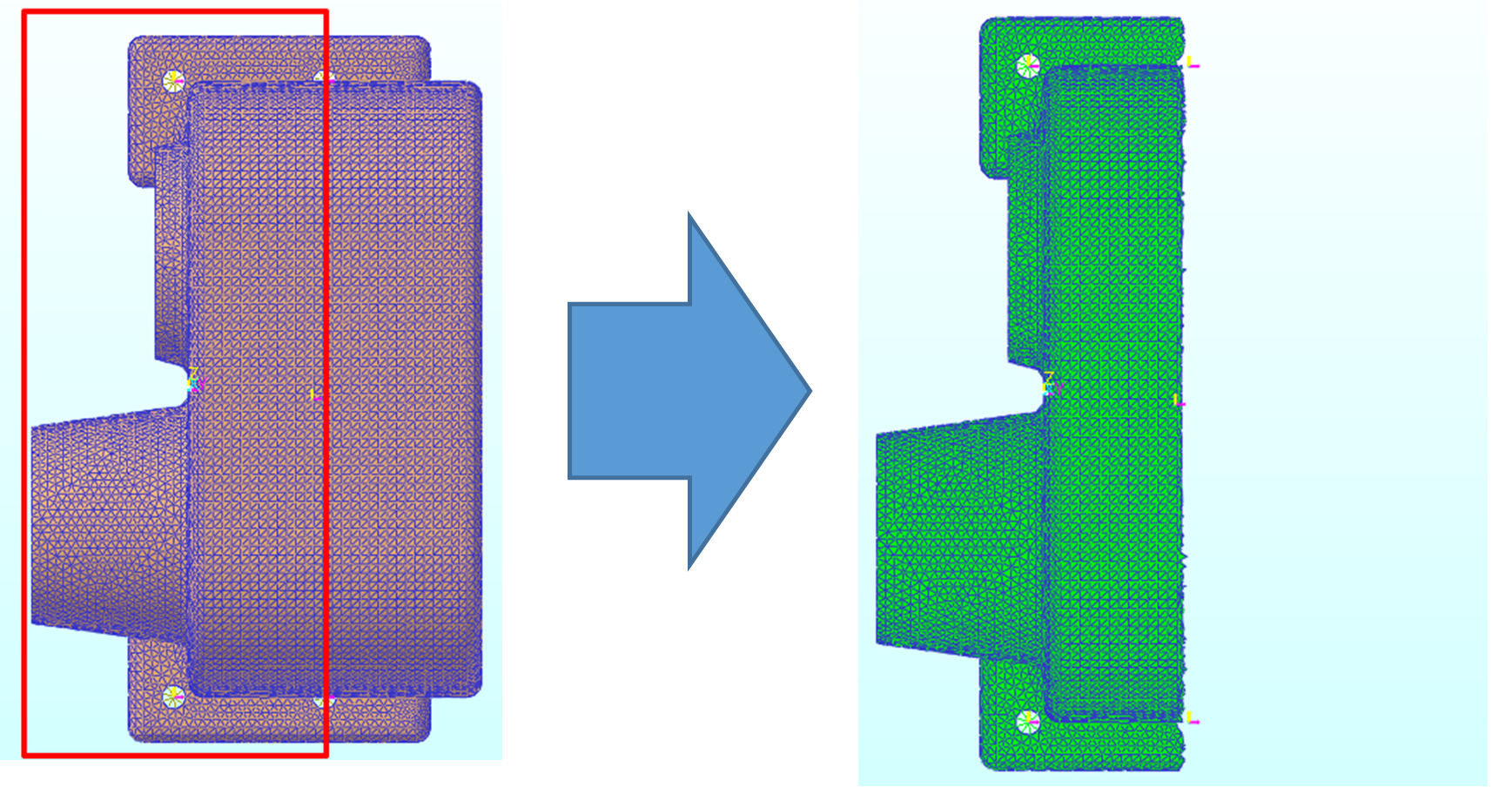
8.1.3.4.1. To create PatchSet:
Enter the Edit Mode of the RFlex body.
Change the plane to the YZ plane.
In Select Toolbar, click the Element tool.
In the working window, select a half of the housing.
In Select Toolbar, click the Set Masking tool.
Only the selected part of the housing will be masked as shown below. Now you can easily select the inside of the housing.
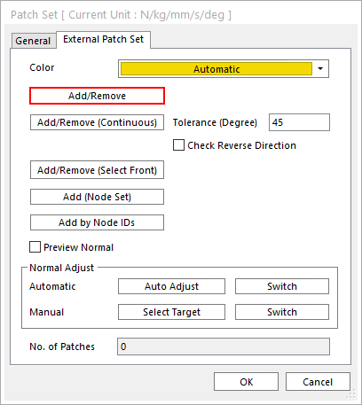
In the Set group of the RFlex Edit tab, click the Patch Set function.
Click Add/Remove (Continuous) in the Patch Set dialog window.
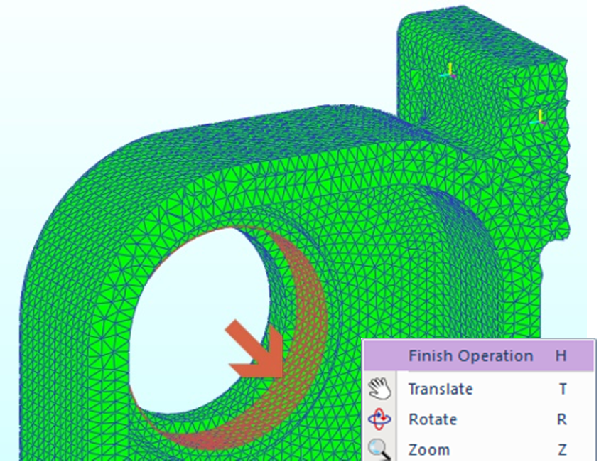
Select the upper bearing position as shown on the below.
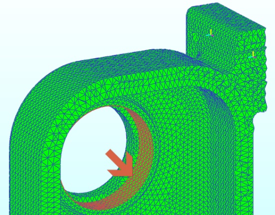
Right-click the working window and click Finish Operation in the pop-up menu.
Click OK in the Patch Set dialog window.
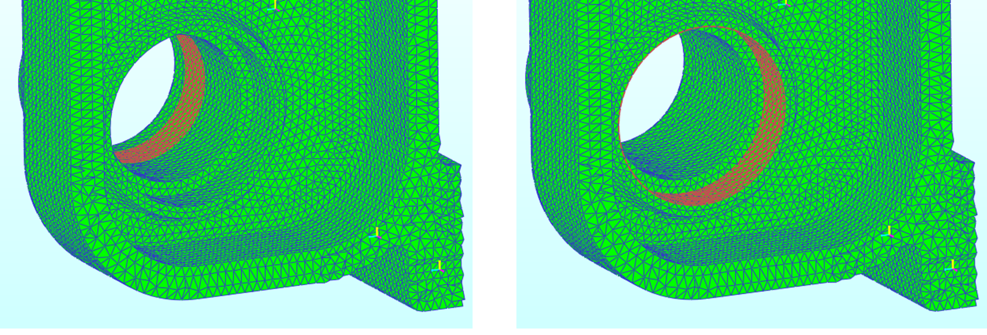
Repeat steps 3 to 10 to create a patch set in other bearing positions as shown below.
In Select Toolbar, click the Set Reverse Masking tool.
Only except for the selected part above will be masked as shown below.
Repeat steps 3 to 10 to create a patch set in other bearing positions as shown to the below.
When the four patch sets are created, click the Cancel Masking tool on Select Toolbar.
Click the Exit function to exit the Edit Mode.
8.1.3.4.2. To create Geo Surface Contact:
On the Flexible tab, in the RFlex group, click the Geo Surface Contact function.
Change the Creation Method to Surface(PatchSet), Surface(PatchSet).
Click the Layer Settings tool in Render Toolbar.
In the Layer Settings dialog window, check On only for the UpperBearing.
In the working window, click UpperBearing1.ImportedSolid1.Face3.
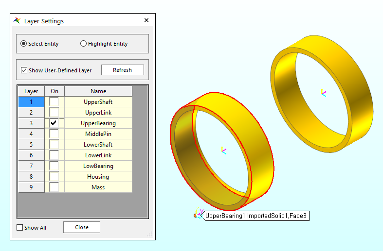
In the Layer Settings dialog window, turn off UpperBearing and ensure that only the housing is visible.
Click the patch set of the housing suitable for the position of bearing selected in 5.
GeoSurContact1 is created.
Repeat steps 1 to 7 to create a contact in the remaining bearing positions.
8.1.3.4.3. Modifying the property of GeoSurContact
In the Database Window, select GeoSurContact1, GeoSurContact2, GeoSurContact3, and GeoSurContact4 and open the Multi-Properties dialog window.
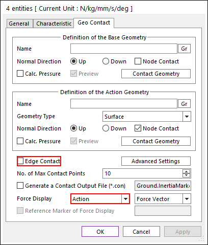
Turn off the Edge Contact option.
Set the Force Display as Action.
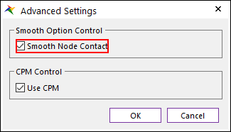
Click Advanced Setting.
In the Advanced Setting dialog window, turn on Smooth Node Contact and press OK.
Move to the Characteristic page on the Multi-Property dialog window.
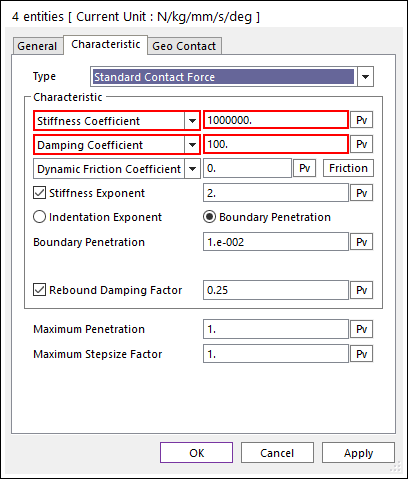
Modify Stiffness Coefficient to 1000000.
Modify Damping Coefficient to 100.
8.1.3.4.4. To save the model:
Save the model as VibratingTransmission_RFlex.rdyn.
8.1.3.5. Performing Simulation
Run simulation to see if the model has been properly converted to a RFlex body.
8.1.3.5.1. To run the simulation:
On the Analysis tab, in the Simulation Type group, click the Dynamic Kinematic Analysis function. The Dynamic/Kinematic Analysis dialog window appears.
Confirm the settings.
On the General page, set as follows:
End Time: 0.1
Step: 500
On the Parameter page, enable the option Match Solving Stepsize with Report Step.
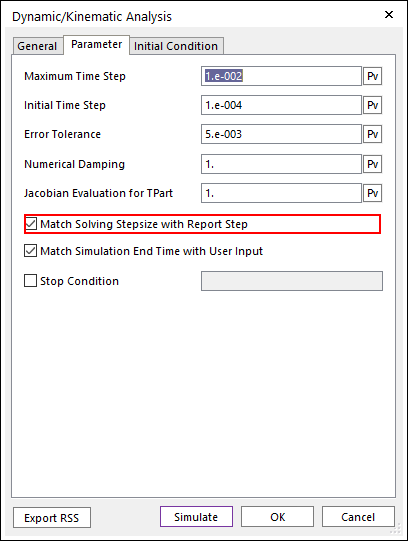
In the next chapter, when calculating the FFT of the ERP, the data is divided at an equal interval. So you can use this option to produce better results.
Click Simulate.
8.1.3.5.2. To view the stress contour result:
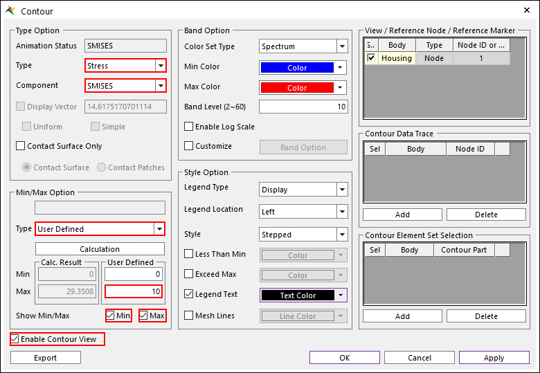
On the Flexible tab, in the RFlex group, click the Contour function.
In Contour Option group, set the Type to Stress.
In Contour Option group, set the Component to SMISES.
In Min/Max Option group, set the Type to User Defined.
Click Calculation.
Change Max to 10.
Select the Show Min/Max checkbox.
Click OK.
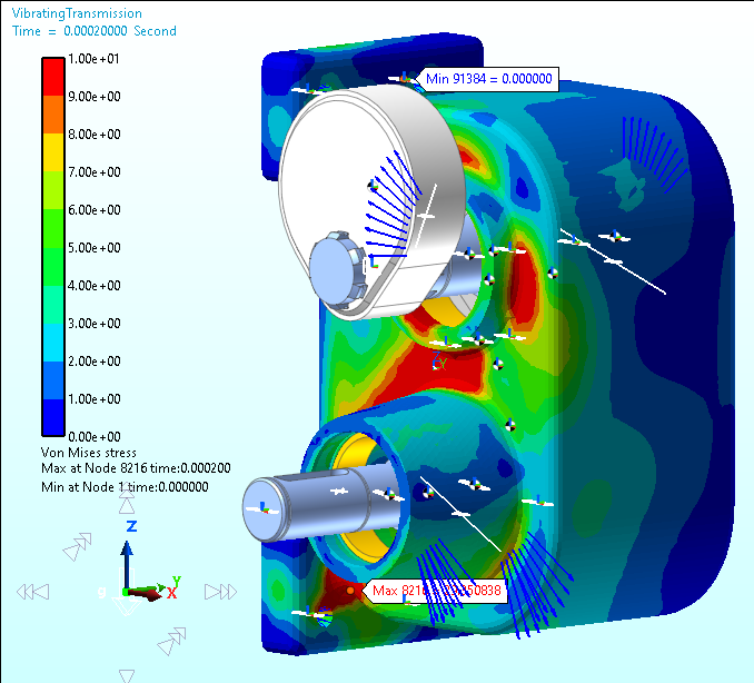
8.1.3.5.3. To view animation:
On the Analysis tab, in the Animation Control group, click the Play function to check the result of stress. At 0.0548 seconds, you can see that the result of Maximum Von-Mises Stress is approximately 20 Mpa.
8.1.4. Calculating Equivalent Radiated Power
The Acoustics analysis is a post tool and can be performed at any time with the analysis result of a flexible body (FFlex, RFlex). In the case of RFlex body, ERP can be additionally calculated for each mode, so you can analyze which mode affects it the most.
8.1.4.1. Task Objectives
In this chapter, you will learn how to calculate the ERP (equivalent radiated power) results using the functions provided by RecurDyn/Acoustics, and to derive the results through Scope and Contour.
8.1.4.2. Estimated Time to Complete This Task
15 minutes
8.1.4.3. Viewing Acoustics Result
Acoustics analysis is carried out using the result simulated in Chapter 3. Before proceeding with the analysis, you should set the range for calculating ERP using a patch set.
What is ERP (equivalent radiated power)?
One of the methods to analyze the frequency response of surface vibrations in a flexible body is to analyze the ERP results.
ERP is the sum of vibration energy generated from the surface as shown in the following equation.
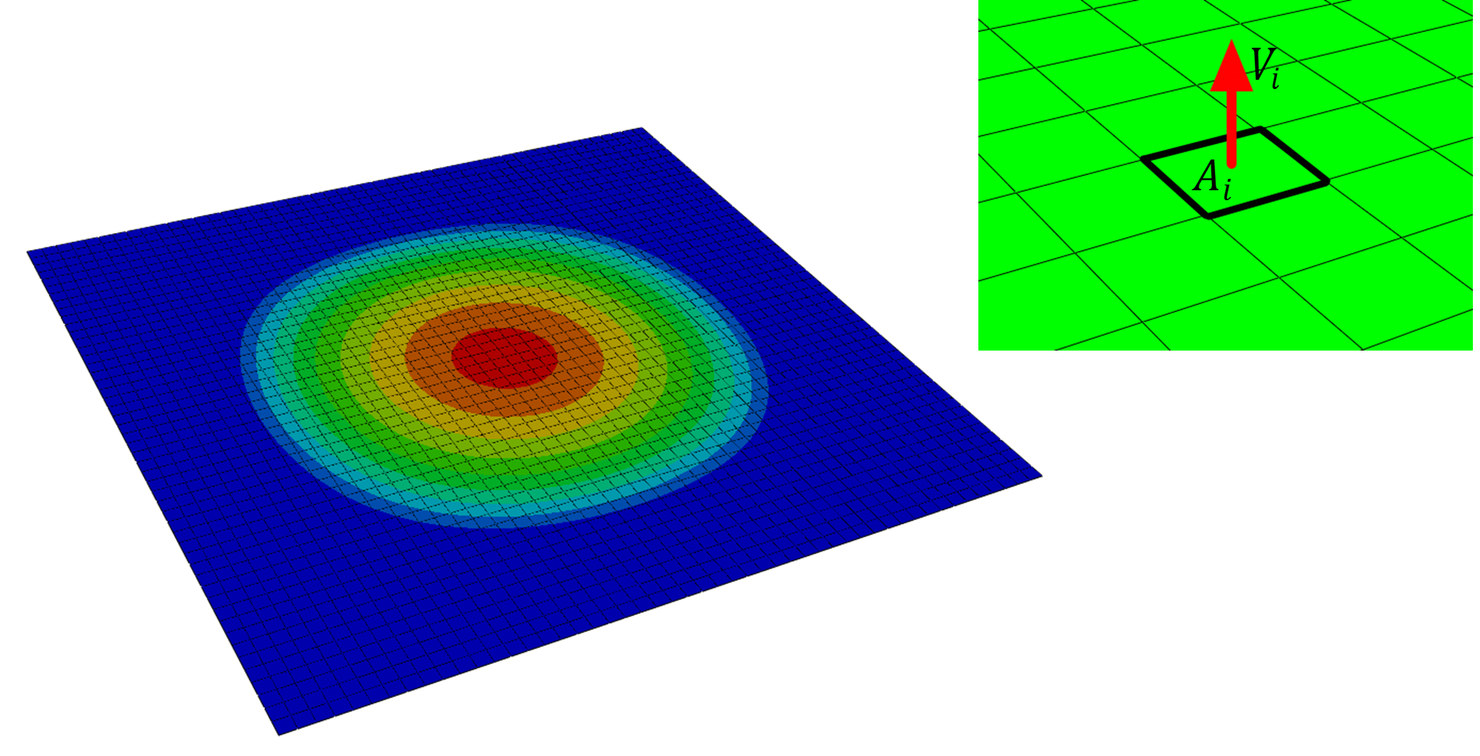
\(ERP = RLF*\left( \frac{1}{2} \right)*C*RHO*\sum_{}^{}\left( A_{i}*{V_{i}}^{2} \right)\)
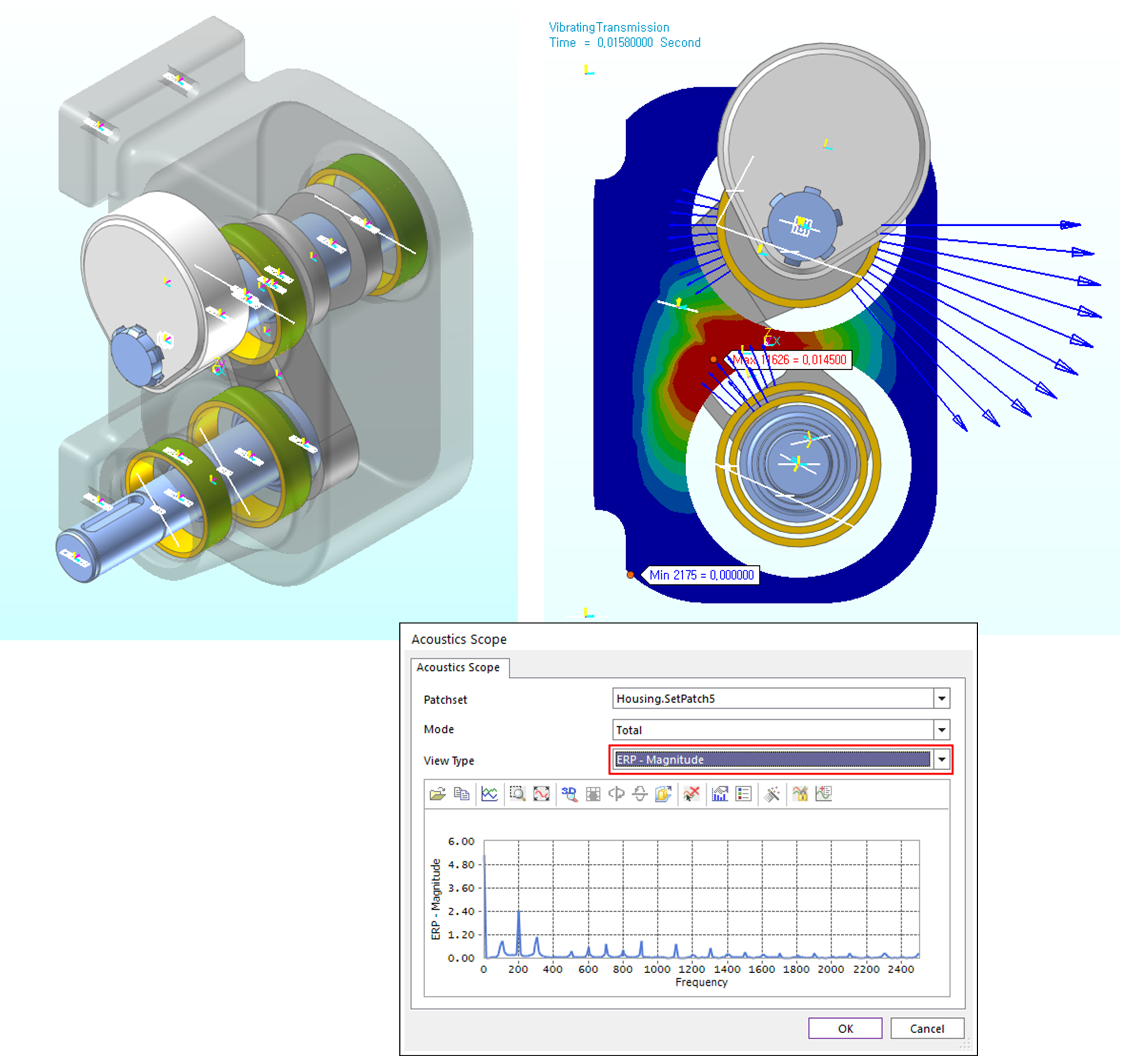
RecurDyn calculates the ERP by calculating the area and vertical velocity of each element for a specific patch set defined by the user. The ERP results for time domain and the results of using FFT (Fast Fourier Transform) as frequency domain are provided through Acoustic Scope. You can also check the ERP results using Contour animation.
8.1.4.3.1. To create a patch set for Acoustics calculation:
Enter the RFlex Edit mode of the Housing.
In the Set group of the FRFlex Edit tab, click the Patch Set function.
In Tolerance (Degree), enter 1.
Click Add/Remove (Continuous) in the Patch Set dialog window.
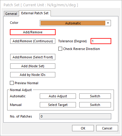
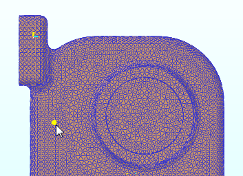
Click the side of the housing as shown on the below. The entire side is selected.
Right-click the working window and click Finish Operation in the pop-up menu.
Click OK in the Patch Set dialog window. SetPatch5 is created.
Click the Exit function to exit the Edit Mode.
8.1.4.3.2. To reload an animation:
In the process of creating the patch set, the relationship between the model and the animation is lost. Click Reload the Last Animation file to retrieve the animation data to the model again.
(If the reload is not possible, import the RAD or RAN file directly from the analysis result folder.)
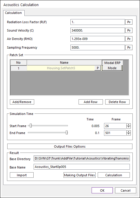
8.1.4.3.3. To calculate Acoustics:
On the Post Analysis tab, in the Acoustics group, click the Acoustics Calculation function. The Acoustics Calculation dialog window appears.
Since the simulation was performed at 500 steps per 0.1 second, you can extract the 5000 Hz result.
Modify Sampling Frequency to 5000. Sampling frequency is used in the process of performing FFT for ERP.
In order to add a patch set, click Add/Remove.
In the working window, select Housing.SetPatch5 created right before.
Right-click the working window and click Finish Operation in the pop-up menu.
Set the Start Frame to 1 and End Frame to 501, which is the endmost value.
Set Base Name as Acoustics.
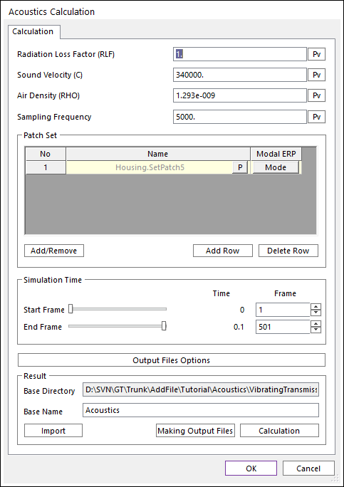
Click Calculation.
When the calculations are complete, click OK to close the dialog window.
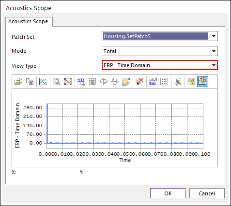
8.1.4.3.4. To view Acoustics scope:
On the Post Analysis tab, in the Acoustics group, click the Acoustics Scope function.
- Change the View Type to ERP-Time Domain.Scope shows the ERP calculation result of time domain for the whole housing.There is a section that is not related to the periodic motion in the stabilizing phase between 0 and 0.005 seconds. In order to proceed with the FFT clearly, the ERP must be calculated again after removing the corresponding interval.
Click Cancel to close the Acoustics Scope dialog window.
8.1.4.4. Viewing Acoustics Results for Modal ERP
We will calculate the ERP for each mode of a RFlex body and analyze which mode has the greatest effect on the total ERP.
8.1.4.4.1. To recalculate Acoustics considering the modal ERP:
On the Post Analysis tab, in Acoustics group, click the Acoustics Calculation function. The Acoustics Calculation dialog window appears.
Click Mode of the Housing.SetPatch5 previously selected.
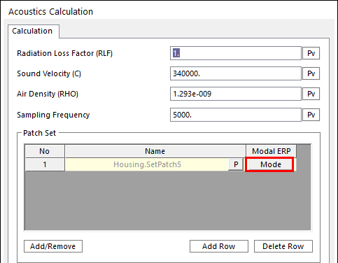
The Mode Selection dialog window appears.
Select the Mode numbers 7, 8, and 9 and click Close.
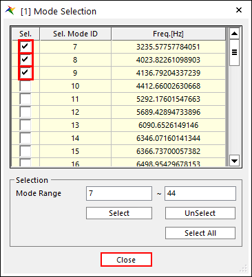
Set Start Frame to 26 to calculate starting from 0.005 second to eliminate the interval that seems not related to the periodic motion between 0 second and 0.005 second.
Change Base Name to Acoustics_Start0p005.
Click Calculation.
When the calculations are complete, click OK to close the dialog window.
8.1.4.4.2. To view Acoustics scope:
On the Post Analysis tab, in the Acoustics group, click the Acoustics Scope function.
Change the View Type **to **ERP-Time Domain.
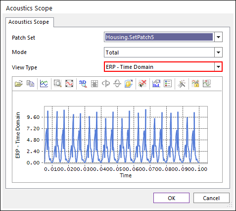
Time Domain ERP calculations are removed for up to 0.005 second, so they are well organized into the analytical data.
Change the View Type to ERP-Magnitude.
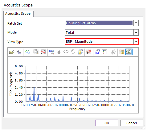
It can be seen that the harmonic frequency occurs for the 100Hz frequency.
Change the mode to analyze the results for Total, Mode7, Mode8, and Mode9.
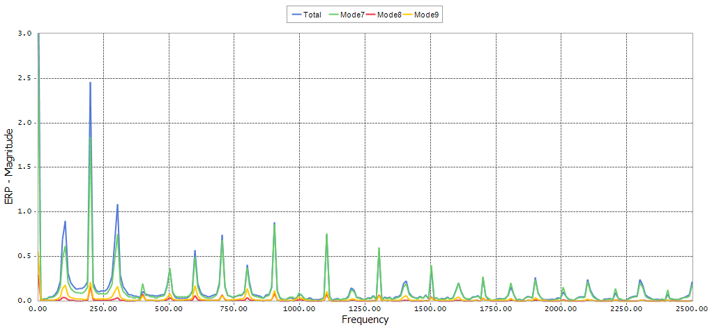
If ERP-Magnitude is plotted against Total, Mode7, Mode8, and Mode9 at once, you can see that Mode7 has the greatest effect.
Click Cancel to close the Acoustics Scope dialog window.
8.1.4.4.3. To view the Acoustics Contour result:
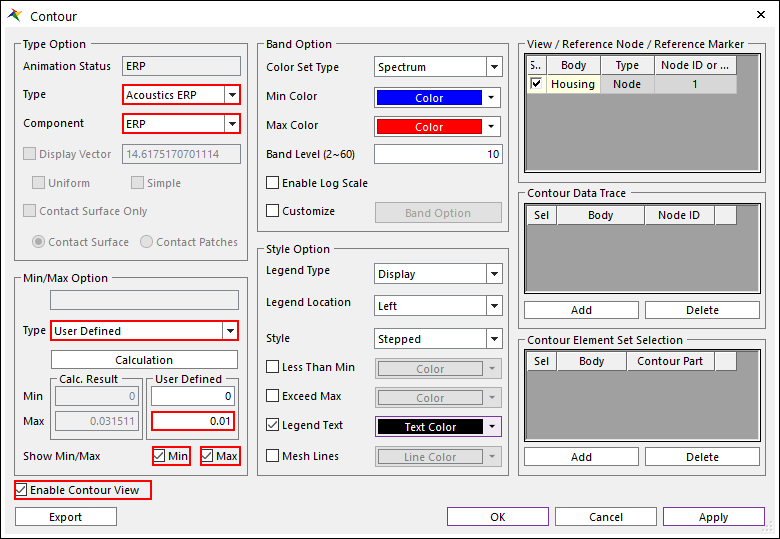
On the Post Analysis tab, in the Acoustics group, click the Acoustics Contour function.
Set the Type to Acoustics ERP.
Set the Component to ERP.
In Min/Max Option group, set the Type to User Defined.
Click Calculation.
Set Max to 0.01.
Select the Show Min/Max checkbox.
Click OK.
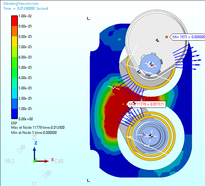
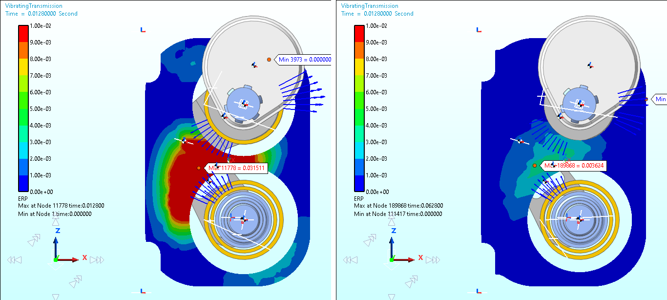
On the Analysis tab, in the Animation Control group, click the Play function to check the result of ERP. The Contour result shows that the ERP value is biggest in the middle part.
Again, open the Contour dialog window and draw an ERP Contour for other Modes.
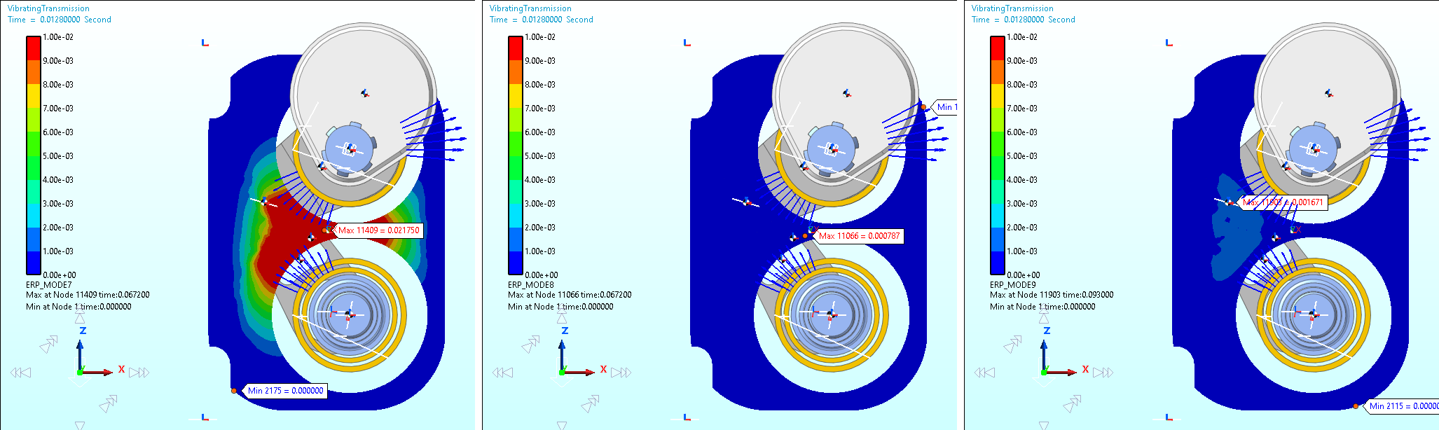
The ERP_HOUSING_MODE7 result is similar to the Total result, and the rest of the modes is considered to have no significant impact.
8.1.5. Modifying and Analyzing the Model
8.1.5.1. Task Objectives
We will try to improve the model so that the noise vibration generated in the housing can be reduced.
8.1.5.2. Estimated Time to Complete This Task
15 minutes
8.1.5.3. Replacing the Housing
8.1.5.3.1. To replace with a RFlex body:
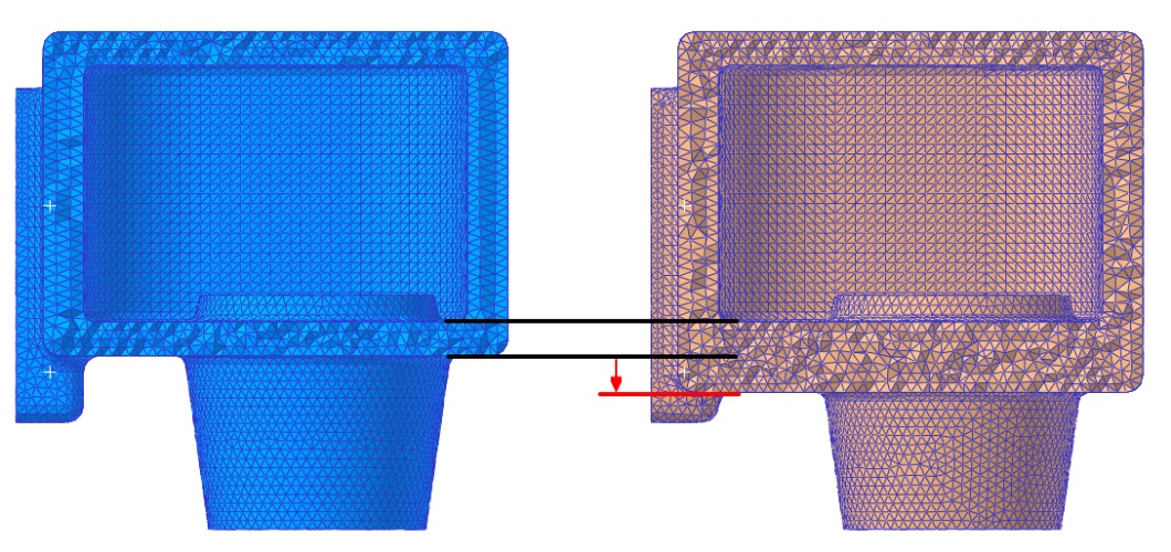
Repeat the procedure for swapping with the RFlex body that you carried out in Chapter 3. For the RFlex body to replace the housing, use the file Housing_Modified.rfi in the folder copied in Chapter 2.
The thickness of the housing has been modified to reduce noise on the sides. Comparing it with the existing housing produces the following figure.
8.1.5.3.2. To redefine contact:
Repeat the procedure in Chapter 3 to redefine contact.
8.1.5.3.3. To save the model:
Save the model as VibratingTransmission_RFlex_NewHousing.rdyn.
8.1.5.3.4. To perform simulation after saving the model:
Execute the simulation in the same conditions as those simulated in Chapter 4.
8.1.5.4. Viewing the Acoustics Result
Repeat the Acoustics calculation procedure in Chapter 4 to calculate the ERP for the side of the housing again.
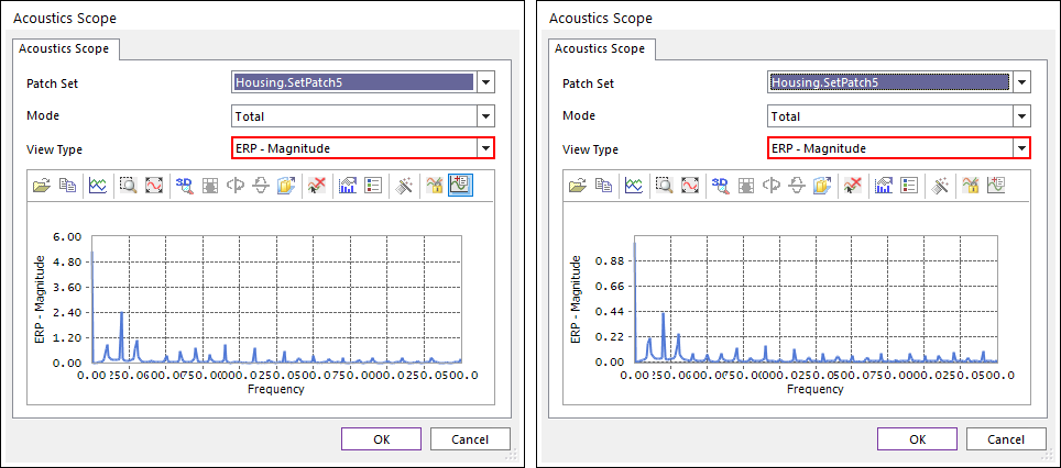
Note that the ERP-Magnitude value at 200 Hz is reduced from 2.4 to 0.42.