3.5. Paper Feeding System Tutorial (AutoDesign)

3.5.1. Outline of Tutorial Sample E

Model

Description

Sample E

Paper Feeding System Design Problem: When a paper feeds through the roller system-2 and pass through the roller system-1. In a given time, the roller system-1 rotates reversely. Then, the paper runs the roller system-1 backward. The design goal is to minimize the slip between roller-system and paper while satisfying the nip force limitation. Key Point: Study the Expression for representing the slip phenomenon. Also, note the design modeling approach to use the guide position as design variable.

3.5.2. Paper Feeding System Design Problem

A paper feeds into the roller system-2 and runs through the roller system-1. When the end of paper passes at the event sensor position, the rotation direction of the roller system-1 is changed as reverse direction.

The design objective is to minimize the slip amount between the paper and the fixed roller in the roller system-1 while satisfying the nip forces of two roller systems for their limits.

The design variables are the stiffness, damping and pre-load of nip springs and the rotation angle of the guide attached in the green colored dummy body.

Open files related in Sample-E
Sample	<InstallDir>\Help\Tutorial\AutoDesign\PaperFeedingSystem\Examples\Sample_E.rdyn
Solution	<InstallDir>\Help\Tutorial\AutoDesign\PaperFeedingSystem\Solutions\Sample_E.rdyn

Note

If you change the file path at discretion, it can be located in any folder that you specify.

3.5.3. Loading the Model and Viewing MTT2D Model

3.5.3.1. To load the base model and view the animation:

1. On your Desktop, double-click the RecurDyn tool. RecurDyn starts and the Start RecurDyn dialog box appears.

2. Close Start RecurDyn dialog box. You will use an existing model.

3. In the Quick Access toolbar, click the Open and select Sample_E.rdyn from the same directory where this tutorial is located.

4. The paper feeding system appears in the modeling window. Click the center of model to switch model as MTT2D.

5. Click Dynamic/Kinematic.

6. Click Simulate.

7. In order to view result, click Play.

   The paper moves from left upper end to the right bottom end. The paper will hit the guides during it progresses.
   

3.5.4. Defining the Design Variables

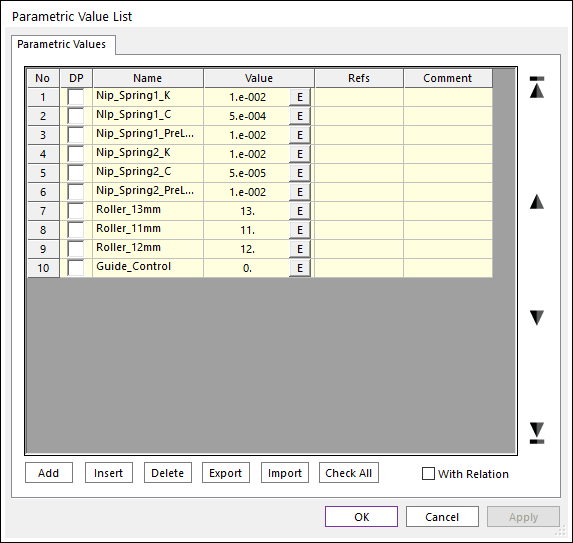
When you see the Parametric Value in the SubEntity menu, the following 10 parameters are listed. Among them, parameters 1~6 and 10 are the design variable.

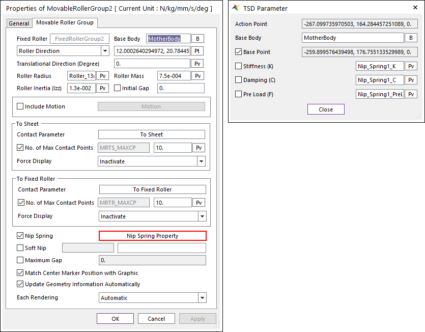
The nip spring properties are linked to the parametric values as follows: Check property of MovableRollerGroup2. Then, Nip Spring Property button is activated. Then, click the button. The below window will be shown. Then, define the Stiffness, Damping, and Pre Load by using the parametric values.

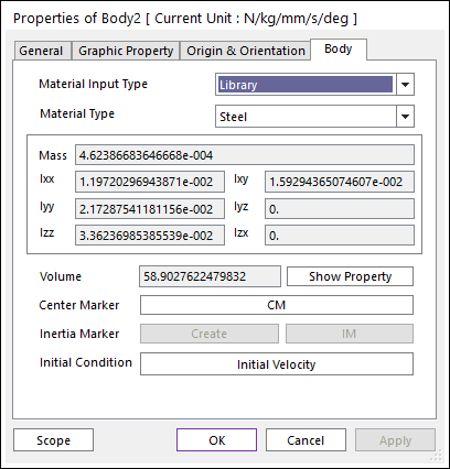
Next, verify the dummy body as Body2 and the Linear Guide to the dummy body.

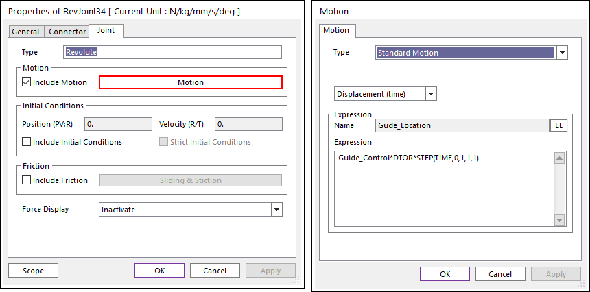
And check the rotational joint at the right end of Body2. This is used only to define the Motion. The parametric value of Guide_Control is used to describe the Motion expression. When the analysis start, the body is rotated with the magnitude of Guide_Control(deg.). Then, the guide will rotate with the same degree because it is attached to the Body2.

3.5.5. Defining the Analysis Response

Although MTT2D provides the mean slips of each roller, they cannot be directly controlled in the Expression, which represents that they are not Analysis Response.

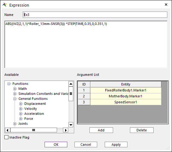
Thus, we make the slip amounts by using the Expression. The below Expression is the slip amount between the paper and the Fixed_roller body in 0.35 second.

The Nip force can be represented by using the spring force.

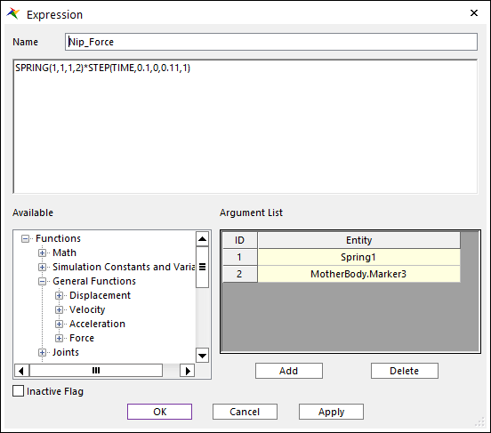
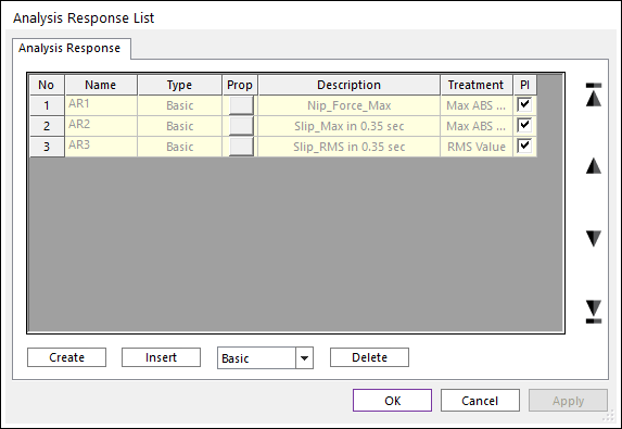
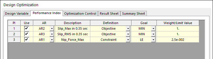
In Analysis Response, the analysis responses are defined as shown the figure below. AR1 is the maximum value of the nip spring force. AR2 is the absolute maximum and AR3 is the RMS of the expression, Ex3.

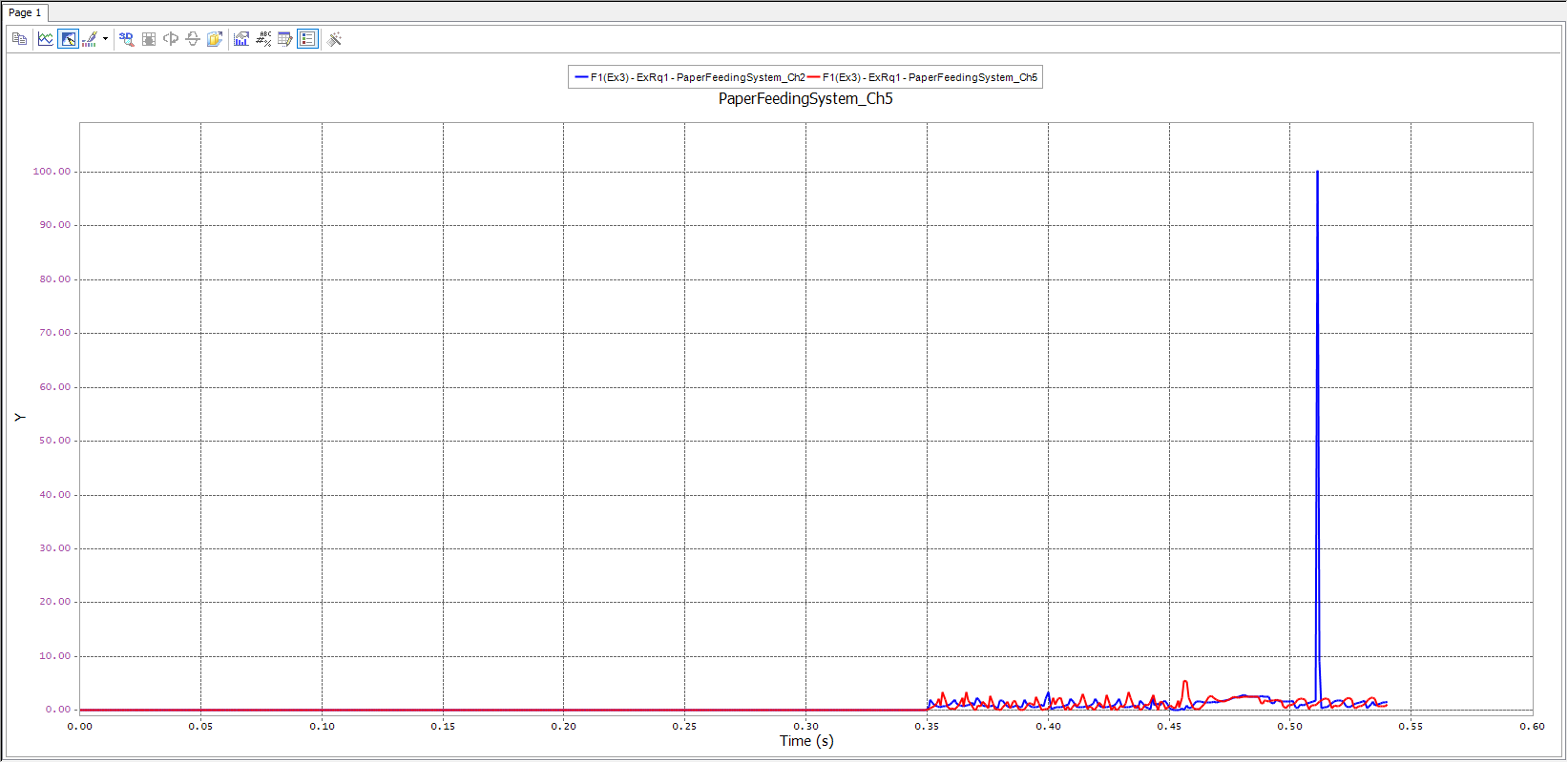
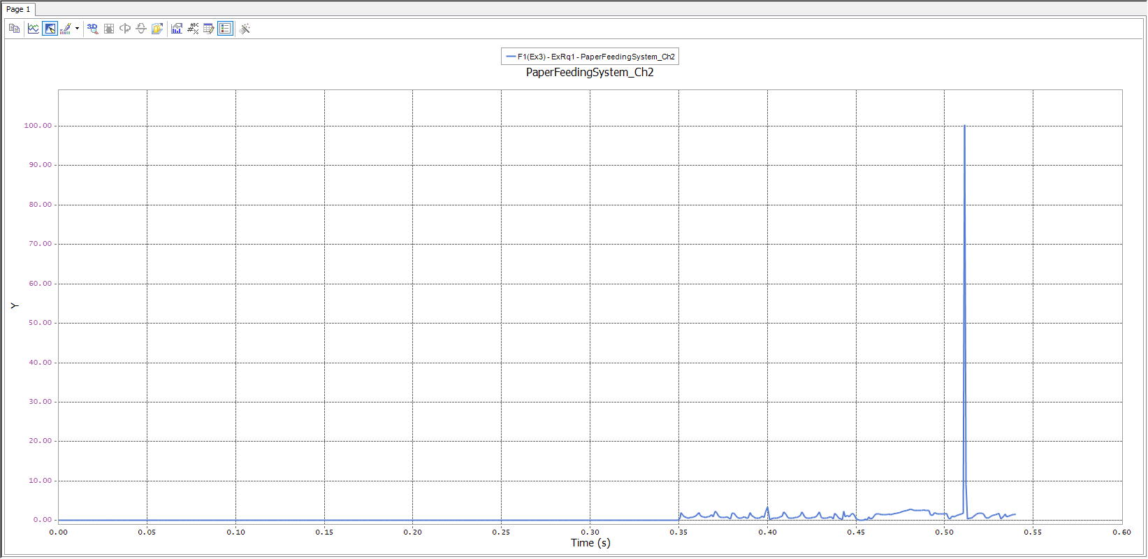
For the initial design, the expression Ex3 gives the following result, which may be highly nonlinear to the change of design variables.

3.5.6. Running a Design Optimization Problem

3.5.6.1. The optimization problem is defined as:

Minimize the Maximum Peak of Slip and the RMS of Slip

subject to

Nip Force =< Limit

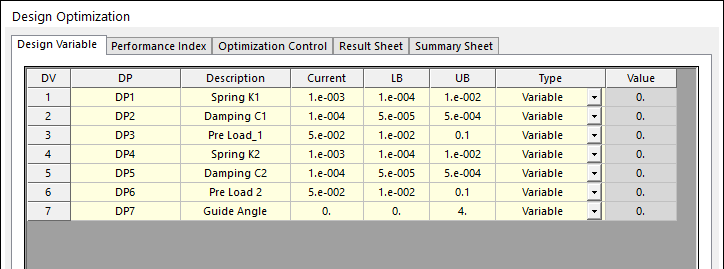
1. In the Design Optimization menu, the Design Variable page shows the list of design variables.

   

2. In the Performance Index page, the above design formulation is defined as below. In this study, the limit of Nip force is used as 0.025(N/mm).

   

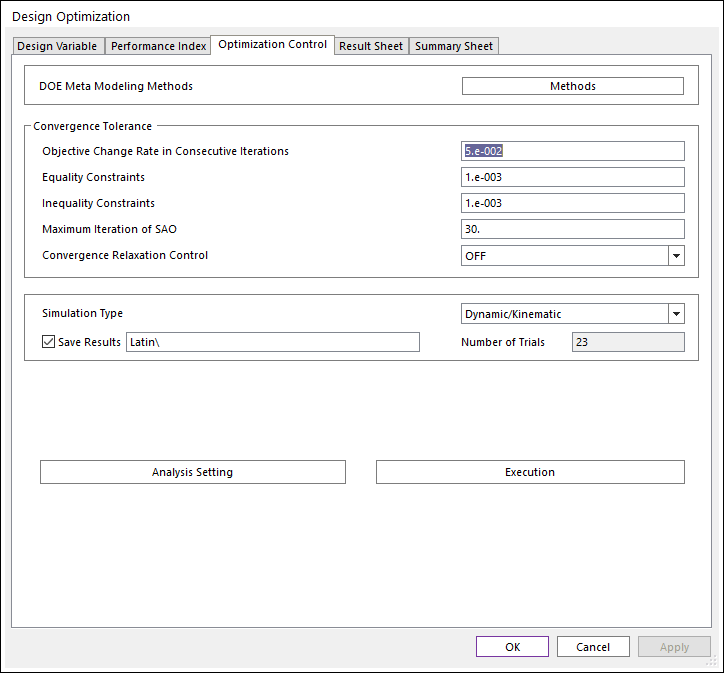
3. In the Optimization Control page, the convergence tolerances use the default values. Push Execution for optimization analysis.

   

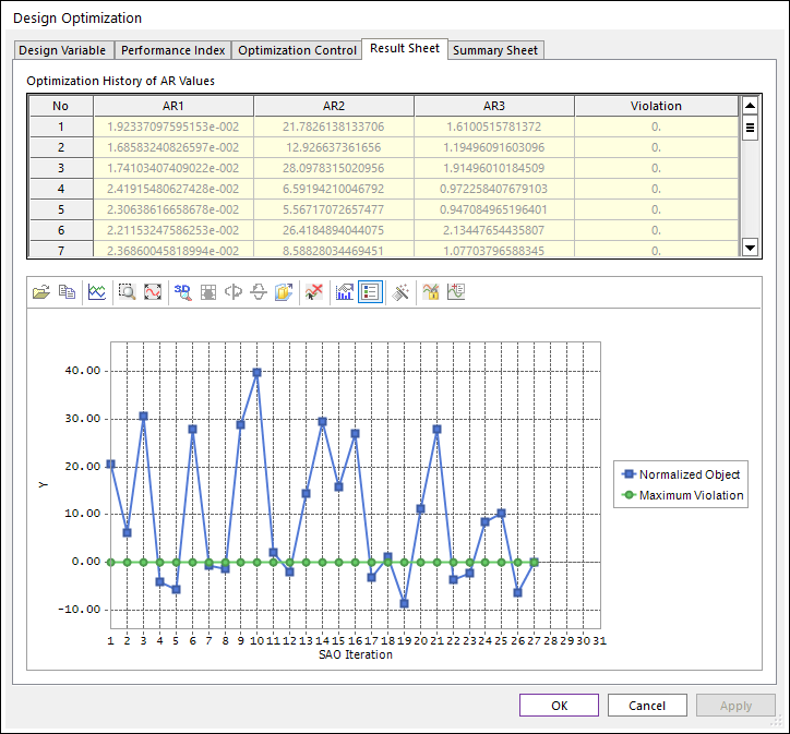
4. Next, check the Result Sheet after the optimization is completed. AutoDesign is converged in 19 iterations. In the final design, the nip force is 0.0248 and the slip amounts such as the maximum peak and the RMS value are 4.44 and 0.955.

   
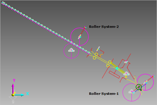
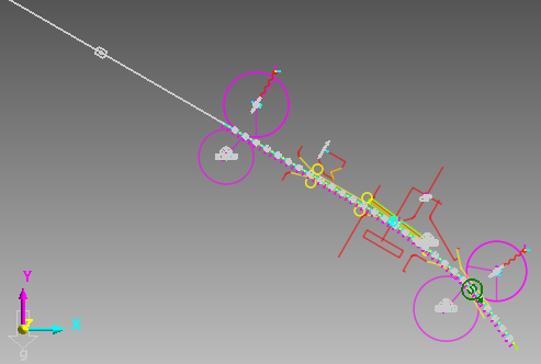
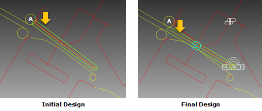
5. The Following figures compare the guide positions for the initial and the final designs. When the paper is reversely feed, the initial design hits the guide marked A but the final design does not.

   Thus, the final design can reduce the slip.
   

3.5.7. Comparison of Analysis Results

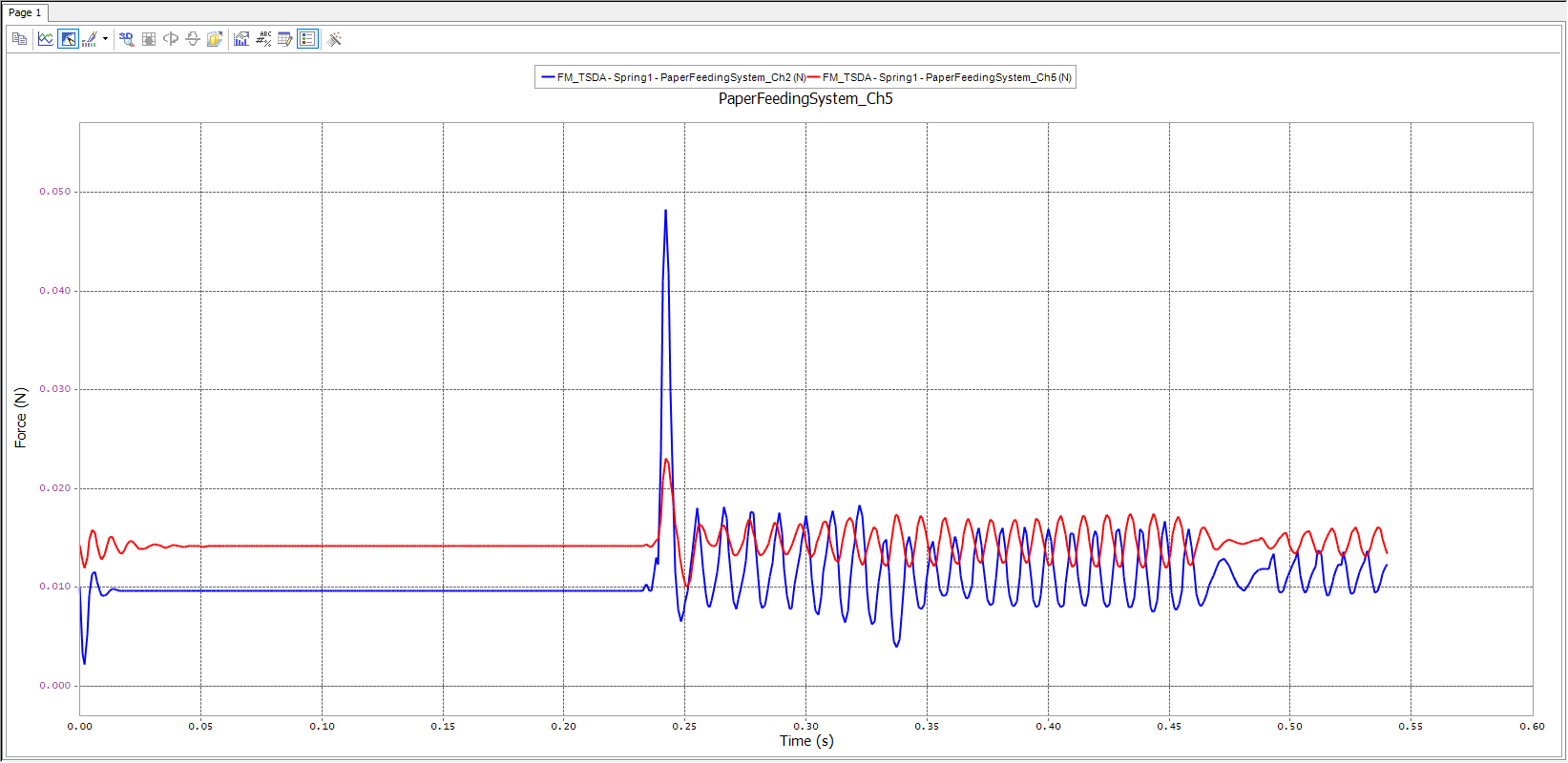
Now, we compare the analysis responses. First, compare the nip forces. The blue color line is the initial design and the red color line is the final design. This comparison shows that the final design satisfies the limitation.

Next, let’s compare the slip amounts. The final design (red color line) is much less than the initial one (blue color line). From our empirical experience, the maximum slip peak, shown as sharply shaped mountain, is highly nonlinear. Thus, its approximation requires many sampling points. Although the shape of the nip forces seems to be sharp, it is however slightly nonlinear because their shapes have same trends according to the changes of design variables. The reason of non-smoothness of the maximum peak of slip amounts is due to the position of guide (DV7). Compare the guide position for the initial and the final design, which explains the non-smoothness.