5.1.1. Property

5.1.1.1. General Page

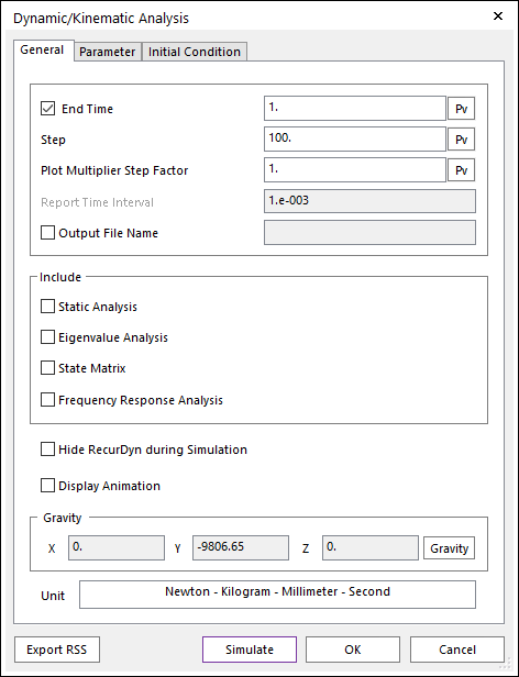
Figure 5.2 Dynamic/Kinematic Analysis dialog box [General]

• End Time: Defines the end time of the simulation. If this option is not checked, the model can be simulated indefinitely. The result data is reported every time set in the Report Time Interval option. If you want to stop the simulation, click Stop.

• Step: Defines the number of data sets for reporting and determines step size of the simulation.

  Note

  RecurDyn/Solver does not interpolate output data to fit the number of Step. If Step is too big, the number of output data from RecurDyn/Solver may be smaller than the defined number. To get the more output data, try reducing the maximum step size.

• Plot Multiplier Step Factor: Defines the number of sampling plot data.

  • The number of sampling plot data = Step * Plot Multiplier Step Factor

  • For example, if Step is 100 and Plot Multiplier Step Factor is 2, the number of sampling plot data is 200.

• Report Time Interval: Defines the interval time for reporting output data. When using endless simulation, the result data is reported every time set in this option.

• Output File Name

  • If this option is checked, it allows defining the model output file name before simulation.

  • If this option is not checked, the output file name is the file name. (The default is unchecked.)

• Include

  • Static Analysis: If this option is checked, a static analysis is performed prior to a dynamic analysis. For more information, refer to Static Analysis.

  • Eigenvalue Analysis: If this option is checked, an eigenvalue analysis is performed at each report time during a dynamic analysis. For more information, refer to Eigenvalue Analysis.

  • State Matrix: If this option is checked, a state matrix is created upon completion of a dynamic analysis. When the Include State Matrix is also selected in the Frequency Response Analysis dialog box, then this option is ignored and the state matrix of Frequency Response Analysis is reported. For more information, refer to State Matrix.

  • Frequency Response Analysis: If this option is checked, a frequency response analysis is performed upon completion of a dynamic analysis. For more information, refer to Frequency Response Analysis.

• Hide RecurDyn during Simulation: If this option is checked, the RecurDyn program window is hidden during the simulation. This allows for faster analysis. By clicking the right mouse button on the RecurDyn icon at the tray, the user can stop the simulation or activate the RecurDyn main window.

  

  Figure 5.3 Hide RecurDyn during Simulation

• Display Animation: If this option is checked, an animation is displayed during the simulation process.

• Gravity: Defines the direction and magnitude of the gravity force.

• Unit: Shows the using unit in the current model.

• Export RSS: Exports the RSS file as the current option.

5.1.1.2. Parameter Page

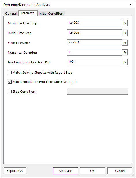
Figure 5.4 Dynamic/Kinematic Analysis dialog box [Parameter]

• Maximum Time Step: Defines the upper bound time step size of the integrator during the dynamic analysis. Since RecurDyn uses variable step size, the step size changes during simulation. Too small maximum time step can slower the simulation speed.

  

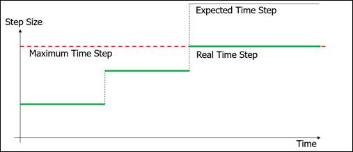
  Figure 5.5 Maximum Time Step

• Initial Time Step: Defines the initial time step of the integrator during the simulation. In most of the cases, the default value 1.e-6 is good enough.

  

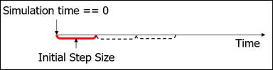
  Figure 5.6 Initial Time Step

• Error Tolerance: Defines the error term used during the simulation process. The system equations are solved using a Newton-Raphson method. The Newton Raphson has converged when norm of \(\delta q\) is less than a specified Error Tolerance. Small error tolerance makes the simulation stricter. In most of the cases, you can use the default value.

  • \(Residual=-Jacobain*\delta q\)

  • \(q\): Vector of Generalized Coordinates

• RecurDyn solves the equations of motion for general systems

  

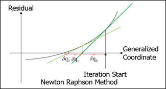
  Figure 5.7 Newton Raphson Method

• Numerical Damping: Defines the damping ratio for the generalized alpha method [4]. Parameters of Generalized-Alpha method are all a function of the numerical damping (ND). This can cause the damping effect even if there is no damper in the system. ND is required to be in the range 0<=ND<=1.

  • ND = 0 implies no numerical damping, and ND = 1 implied maximum numerical damping.

  • In real system, there are several kinds of damping effects which cannot be included in the model, so in most of the cases you can use the default value

• Jacobian Evaluation for TPart: In the Tpart included system, you cna control the parameters of jacobian evaluation. The jacobian evaluation means the number of integration steps between each evaluation of jacobian. For example, if the value is 100, the jacobian will be computed once per 100 integration steps. Tpart are track links, chain links, and belt segments.

• Match Solving Stepsize with Report Step: If you check this option, the solving step and report step are coincided. The step size of the animation is uniform (end time/steps). But the real step size of the solver or plot data is non uniform. So, you may not get the simulation result at the specific time instant. (for example, even if you want a result at 1.5s, the solver may calculate 1.47s then the next step can be 1.51 (step size is 0.04s)). By checking this option, the solver calculates the time instants at N*end time/steps and match the animation step and the plot step.

  Note

  Following toolkits use always the Match Solving Stepsize with Report Step option.

  1. TSG

  2. SPI (Standard Particle Interface) - External & Embedded

• Match Simulation End Time with User Input: If you check this option, the simulation is finished at the user-defined End Time. (The default is checked.)

• Stop Condition: If this option is checked, you can define an expression function. If the input expression becomes true, solver is stopped. Here, the value that evaluates to true is a value greater than zero.

  

  Figure 5.8 Stop Condition

  • For example, if Ex1 is inputted to Stop Condition after AZ (1, 2)>40D is made by Expression (Ex1), the value of Ex1 is as follows. For more information, refer to Relational Operators, Logical Operators.

  • If the angular difference to the z axis of the first marker and the second marker is bigger than 40 degrees, the value of Ex1 is 1 and the solver is stopped.

  • If the angular difference to the z axis of the first marker and the second marker is less than 40 degrees, the value of Ex1 is 0.

5.1.1.3. Initial Condition Page

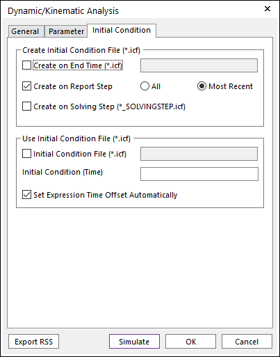
Figure 5.9 Dynamic/Kinematic Analysis dialog box [Initial Condition]

• Create Initial Condition File(*.icf)

  • Create on End Time(*.icf): If you check this option, RecurDyn makes a *.icf file as the specified name at the end time of the simulation.

  • Create on Report Step: If you check this option, you can select the two options.

    • If you select ALL option, RecurDyn makes [Animation Frame]_[Report Time].icf file in the _ICF_[RMD Name] folder at the every reporting time of the simulation. (CAUTION: This option causes the simulation time to be slow.)

    • If you select Most Recent option, RecurDyn makes [model name]_REPORTSTEP.icf file and updates this file at the every reporting time of the simulation.

  • Create on Solving Step: If you check this option, RecurDyn makes [model name]_SOLVINGSTEP.icf file and updates this file at the every solving time of the simulation.

• Use Initial Condition File(*.icf)

  • Initial Condition File(*.icf): If you check this option, RecurDyn imports the *.icf file at the beginning of the simulation process.

  • Set Expression Time Offset Automatically: If you check this option, Solver automatically converts the Time Offset internally to the simulation time saved in the icf file. A warning message about this appears when the simulation starts.