21.3.5.2. Multi-Objective Optimization in RecurDyn/AutoDesign
AutoDesign uses the weighted min-max type preference function. Now, in order to explain the determination of ideal target \(f_{i}^{*}\) for each objective, the following sample problem is introduced.
\(\begin{aligned} & \underset{x}{\mathop{\min }}\,{{f}_{i}}\left( \mathbf{x} \right),\text{ }i=1,2,...,4. \\ & \operatorname{subject}\text{ }to\text{ }-5.0\le {{x}_{k}}\le 5.0,\text{ }k=1,2. \\ \end{aligned}\)
where, \({{f}_{1}}\left( \mathbf{x} \right)=\left( {{\left( {{x}_{1}}-3 \right)}^{2}}+{{\left( {{x}_{2}}-3 \right)}^{2}} \right)\), \({{f}_{2}}\left( \mathbf{x} \right)=\left( {{\left( {{x}_{1}}+3 \right)}^{2}}+{{\left( {{x}_{2}}+3 \right)}^{2}} \right)\),
\({{f}_{3}}\left( \mathbf{x} \right)=\left( {{\left( {{x}_{1}}-3 \right)}^{2}}+{{\left( {{x}_{2}}+3 \right)}^{2}} \right)*3.0\) and \({{f}_{4}}\left( \mathbf{x} \right)=\left( {{\left( {{x}_{1}}+3 \right)}^{2}}+{{\left( {{x}_{2}}-3 \right)}^{2}} \right)*4.0\).
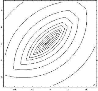
The following figure shows the contour of the composite function, \(\max \left\{ {{f}_{i}} \right\}\).
As you know, AutoDesign uses meta-model to solve the optimization problem. First, it samples 9 points by using ISCD-I. The following table lists the analysis results side by side.
Run |
\({{x}_{1}}\) |
\({{x}_{2}}\) |
\({{f}_{1}}\) |
\({{f}_{2}}\) |
\({{f}_{3}}\) |
\({{f}_{4}}\) |
1 |
5.0 |
-5.0 |
68.0 |
136.0 |
24.0 |
512.0 |
2 |
5.0 |
5.0 |
8.0 |
256.0 |
204.0 |
272.0 |
3 |
-5.0 |
5.0 |
68.0 |
136.0 |
384.0 |
32.0 |
4 |
-5.0 |
-5.0 |
128.0 |
16.0 |
204.0 |
272.0 |
5 |
0.0 |
0.0 |
18.0 |
36.0 |
54.0 |
72.0 |
6 |
5.0 |
0.0 |
13.0 |
146.0 |
39.0 |
292.0 |
7 |
-5.0 |
0.0 |
73.0 |
26.0 |
219.0 |
52.0 |
8 |
0.0 |
5.0 |
13.0 |
146.0 |
219.0 |
52.0 |
9 |
0.0 |
-5.0 |
73.0 |
26.0 |
39.0 |
292.0 |
In the table, the four functions have different minimum points. RecurDyn/AutoDesign selects the minimum values for each objective such as \(\left( 8.0,16.0,24.0,32.0 \right)\). Then, it estimates the ideal target as 45 % of the selected minimum, which are \(\left( 3.6,7.2,10.8,14.4 \right)\). Finally, it checks the deviation of ideal targets. Then, if the deviation is less than a tolerance value, its re-estimates automatically the ideal target is 45% of the minimum of the candidates. In this case, ideal target for all functions is \(1.62\left( =0.45*3.6 \right)\). Then, AutoDesign solves the following multi-objective problems internally:
\(\underset{\mathbf{x}}{\mathop{\min }}\,\max \left\{ {{w}_{i}}\left( \frac{{{{\tilde{f}}}_{i}}\left( \mathbf{x} \right)-1.62}{1.62} \right) \right\},i=1,2,..,4\)
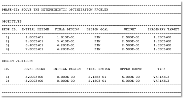
where \({{\tilde{f}}_{i}}\) denotes the ith meta-model constructed from the initial 9 points. It uses an approximate generalized gradient vector for solving the composite non-smooth optimization problem [1]. The following figure shows the inside output of AutoDesign for the given mult-objective problems. It gives an optimum \({{\mathbf{x}}^{*}}=\left( -2.158,2.150 \right)\) and estimated the approximate objectives as \({{\tilde{f}}_{3}}={{\tilde{f}}_{4}}=62.03\).
AutoDesign selects the initial design from the given DOE data. In this case, it uses a weighted summation type preference function.
\(\underset{\mathbf{x}\in \Omega }{\mathop{\min }}\,\sum\limits_{i=1}^{4}{{{w}_{i}}\left( \frac{{{f}_{i}}\left( \mathbf{x} \right)-1.62}{1.62} \right)}\)
where, \(\Omega\) is the given DOE set. The ideal goal is determined automatically. In this problem, it is 1.62.
Reference
M.S. Kim, D.H. Choi, and Y. Hwang, “Composite Nonsmooth Optimization Using Approximate GeneralizedGradient Vectors”, Journal of Optimization Theory and Applications, Vol. 112, pp. 145-165, January 2002.
Osyczka, A., Multicriterion optimization in Engineering with FORTRAN programs, Ellis Horwood Limited, Chichester, 1984.