4.7.1.8. Spline

4.7.1.8.1. SPL

The SPL function uses the selected interpolation type in the spline curve. The spline curve function returns the y values for the x variable input through the spline entity. It uses spline curve in x-y direction and linear interpolate in x-z direction. So, if the user wants to smooth surface effect, then data set of z direction must be dense.

Format

SPL(x, z, Curve name, Order)

Arguments definition

x	An input variable for the spline function Generally, this variable is time or a function that returns a real number.
z	An input variable for the spline function The second variable is necessary for three-dimensional spline functions. This variable must be a function that returns a real number. Otherwise, 0 is applied. y1 = f(x,z1), y2 = f(x,z2) z1<z<z2 y = (z-z1)*(y2-y1)/(z2-z1)+y1
Curve name	The name or argument number of the spline data defined by the subentity
Order	The interpolation method for the functions (return the value if 0, return calculation for 1st order differential equation if 1, and return calculation for 2nd order differential equation if 2) dy1/dx = df(x,z1)/dx, dy2/dx = df(x,z2)/dx dy/dx = (z-z1)*(dy2/dx-dy1/dx)/(z2-z1)+dy1/dx

Formulation

\(\text{SPL=}\left\{ \begin{matrix} f(x,spline\_data),\,\,\,\,\,\,\,\,\,\,\,\,\,\, \\ df(x,spline\_data)/dx,\,\,\,\,\, \\ {{d}^{2}}f(x,spline\_data)/d{{x}^{2}}, \\ \end{matrix}\begin{matrix} \,\text{Order=0} \\ \text{Order=1} \\ \text{Order=2} \\ \end{matrix} \right.\)

Example

SPL(time-4,0,1,0) <Argument: (1) Spline>

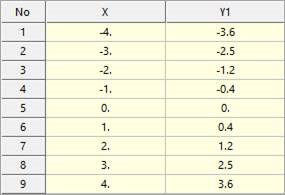
Figure 4.46 Spline Data

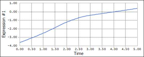
Figure 4.47 Example using the SPL function, selected interpolation type is Akima

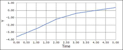
Figure 4.48 Example using the SPL function, selected interpolation type is Linear

4.7.1.8.2. AKISPL

The AKISPL function uses Akima spline interpolation to return the y values for the x variable input through the spline entity. It uses spline curve in x-y direction and linear interpolate in x-z direction. So, if the user wants to smooth surface effect, then data set of z direction must be dense.

Format

AKISPL(x, z, Curve name, Order)

Arguments definition

x	An input variable for the Akima spline function Generally, this variable is time or a function that returns a real number.
z	An input variable for the Akima spline function The second variable is necessary for three-dimensional spline functions. This variable must be a function that returns a real number. Otherwise, 0 is applied. y1 = f(x,z1), y2 = f(x,z2) z1<z<z2 y = (z-z1)*(y2-y1)/(z2-z1)+y1
Curve name	The name or argument number of the spline data defined by the subentity
Order	The interpolation method for the functions (return the value if 0, return calculation for 1st order differential equation if 1, and return calculation for 2nd order differential equation if 2) dy1/dx = df(x,z1)/dx, dy2/dx = df(x,z2)/dx dy/dx = (z-z1)*(dy2/dx-dy1/dx)/(z2-z1)+dy1/dx

Formulation

\(\text{AKISPL=}\left\{ \begin{matrix} f(x,spline\_data),\,\,\,\,\,\,\,\,\,\,\,\,\,\, \\ df(x,spline\_data)/dx,\,\,\,\,\, \\ {{d}^{2}}f(x,spline\_data)/d{{x}^{2}}, \\ \end{matrix}\begin{matrix} \,\text{Order=0} \\ \text{Order=1} \\ \text{Order=2} \\ \end{matrix} \right.\)

Example

AKISPL(time-4,0,1,0) <Argument: (1) Spline>

Figure 4.49 Spline Data

Figure 4.50 Example using the AKISPL function

4.7.1.8.3. CUBSPL

The CUBSPL function uses Cubic spline interpolation to return the y values for the x variable input through the spline entity. The cubic spline function’s 2nd order differential equation calculation is a curve. As such, it is suitable to use the spline input function for motion. It uses spline curve in x-y direction and linear interpolate in x-z direction. So, if the user wants to smooth surface effect, then data set of z direction must be dense.

Format

CUBSPL(x, z, Curve name, Order)

Arguments definition

x	An input variable for the cubic spline function Generally, this variable is time or a function that returns a real number.
z	An input variable for the cubic spline function The second variable is necessary for three-dimensional spline functions. This variable must be a function that returns a real number. Otherwise, 0 is applied. y1 = f(x,z1), y2 = f(x,z2) z1<z<z2 y = (z-z1)*(y2-y1)/(z2-z1)+y1
Curve name	The name or argument number of the spline data defined by the subentity
Order	The interpolation method for the functions (return the value if 0, return calculation for 1st order differential equation if 1, and return calculation for 2nd order differential equation if 2) dy1/dx = df(x,z1)/dx, dy2/dx = df(x,z2)/dx dy/dx = (z-z1)*(dy2/dx-dy1/dx)/(z2-z1)+dy1/dx

Formulation

\(\text{CUBSPL=}\left\{ \begin{matrix} f(x,spline\_data),\,\,\,\,\,\,\,\,\,\,\,\,\,\, \\ df(x,spline\_data)/dx,\,\,\,\,\, \\ {{d}^{2}}f(x,spline\_data)/d{{x}^{2}}, \\ \end{matrix}\begin{matrix} \,\text{Order=0} \\ \text{Order=1} \\ \text{Order=2} \\ \end{matrix} \right.\)

Example

CUBSPL(time,0,1,0) <Argument: (1) Spline1>

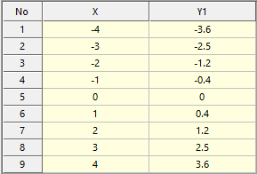
Figure 4.51 Spline Data

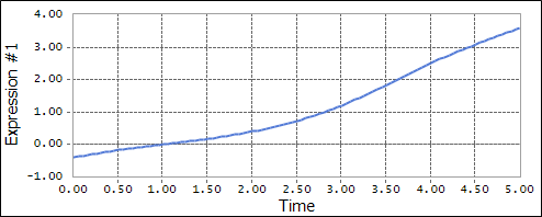
Figure 4.52 Example using the CUBSPL function

4.7.1.8.4. LINSPL

The LINSPL function uses Linear spline interpolation to return the y values for the x variable input through the spline entity.

Format

LINSPL(x, z, Curve name, Order)

Arguments definition

x	An input variable for the linear spline function Generally, this variable is time or a function that returns a real number.
z	An input variable for the linear spline function The second variable is necessary for three-dimensional spline functions. This variable must be a function that returns a real number. Otherwise, 0 is applied. y1 = f(x,z1), y2 = f(x,z2) z1<z<z2 y = (z-z1)*(y2-y1)/(z2-z1)+y1
Curve name	The name or argument number of the spline data defined by the subentity
Order	The interpolation method for the functions (return the value if 0, return calculation for 1st order differential equation if 1, and return calculation for 2nd order differential equation if 2) dy1/dx = df(x,z1)/dx, dy2/dx = df(x,z2)/dx dy/dx = (z-z1)*(dy2/dx-dy1/dx)/(z2-z1)+dy1/dx

Formulation

\(\text{LINSPL=}\left\{ \begin{array}{*{35}{l}} f(x,spline\_data), \\ df(x,spline\_data)/dx, \\ \end{array}\text{ }\begin{array}{*{35}{l}} \text{Order=0} \\ \text{Order=1} \\ \end{array} \right.\)

Example

LINSPL(time-1,0,1,0) <Argument: (1) Spline1>

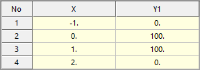
Figure 4.53 Spline Data

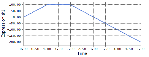
Figure 4.54 Example using the LINSPL function