13.2.1. PMM
PMM is abbreviation of Pidotech Meta Model. The purpose of this function is to make CMM of DNN type (Deep Neural Work) using the technique of Pidotech Meta Model Tool Box. The user inputs the degree of freedom (DOF) for each interface marker and the range of each DOF. Sampling function in order to get random DOE cases are performed. Then, static analysis is performed on the DOE cases at the same time as selecting an option to create a meta model. Finally, meta model files are built based on the result table (DOE cases + response data) automatically. Meta model file can be applied to Component Group.
13.2.1.1. Modeling Options
The user selects the Component Group defined on the model and create CMM of DNN type using the dialog box that appears.
Group
Group: Selects a Component Group using Component Meta Model.
13.2.1.2. The process of creating a Component Meat Model
Component analysis and Creating Component Meta Model proceed through the ComponentGroup dialog that appears when you select a Component Group during the modeling process.
13.2.1.2.1. Component Variable Page
In this page, user create DOE tables. before setting this table, Design Variables should be defined. Here, Design Variables defines the boundary for each DOF.
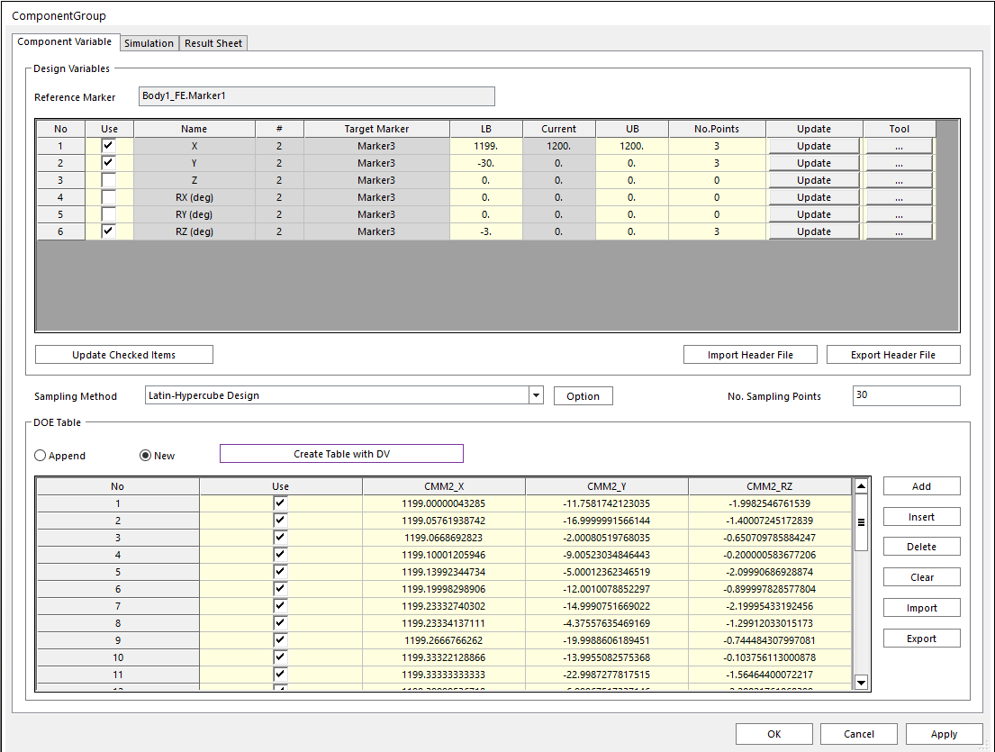
Figure 13.18 Component Variable page in ComponentGroup sheet
Use: If this option is checked, this means using that degree of freedom and creating it in the DOE Table.
LB: Lower boundary of selected DOF.
UB: Upper boundary of selected DOF.
No.Points: The number of points to divide DOF range evenly.
Update: Update the changed contents to the division points.
Tool: Tools to help create points. If you set LB, UB, and the number of points, points are created according to the values.
Update Checked Items: Updates Design variables information to the DOE Table.
Import/Export Header File: Import and export header file(extension mmh) which contains Design Variables Information.
Note
Rx, Ry, Rz in the Design Variables means rotation angle in the direction of x,y and z axis in euler angle ZYX. Refer to EULERANGLE.
Sampling Method: Select Sampling Method in order to make sample points to be the DOE cases.
Latin Hypercube Design (LHD): Generate sample points using LHD method.
Optimization Methiod: Select optimization method for LHD. (Supports opt, rand and auto)
Optimality Criteria: Select Optimality criteria. (Applicable only when Optimization Method is opt)
maximin: Maximize the minimum distance between any two sample points.
entropy: Maximize entropy.
force: Minimize the repulsive force after assuming the experimental points as a charged particles.
Symmetry: Determines whether to maintain symmetry between sample points.
Midpoint in a Cell: Determines whether to maintain position of sample point to the midpoint in a cell.
Repetability: if checked, generate the same sample points every time.
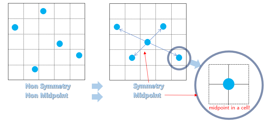
Figure 13.19 Features of Symmetry and Midpoint in a Cell
Fully-Sequential Space-Filling Design (FSSF): Additional sample points are generated based on existing sample points. After generating candidate points that oversaturate the design area, candidate points farthest from the existing sampling points are sequentially selected. Additionally, initial sample points can be generated without existing one.
Create Candidate Points: Select how to generate candidate points that will oversaturate the design area. (lhd: create candidate points with LHD. rand: Create candidate points with Random Sampling)
No. of Candidate Points: Define the number of candidate points that will oversaturate the design space. This value should be more than the additional sampling points user want to get. (if non checked, 1000*nx(=number of design variable) is defined.)
Reflect: Since FSSF tries to select a candidate point farthest from existing experimental points, it has a disadvantage that new experimental points are sampled mainly on the boundary of the design area. Choose whether to use a method to improve these shortcomings.
Repetability: if checked, generate the same sample points every time.
Existing Sampling Data: Import csv file containing existing sample cases.
Expected Improvement-based Sequential Sampling (EISS): Additional sample points are generated based on the existing sample points and their response values.
Repetability: if checked, generate the same sample points every time.
Existing Sampling Data: Import csv file containing existing sample cases and response data.
Note
When the number of sample points is large, obtaining an initial sample points through FSSF shows better performance. (design variable x 1000)
Append: Append DOE cases generated from sampling method.
New: Replace with DOE cases generated from sampling method.
Create Table with DV: Create DOE table based on DOE cases generated by Sampling Methood.
Add: Add row.
Insert: Insert row.
Delete: Delete row.
Cleae: Clear all DOE cases in the tabe.
Import: Import DOE table information.
Export: Export DOE table information.
Note
No. Points is not related to CMM creation of DNN type since random DOE cases are used rather than a DOE cases of full factorial design made of grid points generated by equally dividing each DOF.
13.2.1.2.2. Simulation Page
In this page, user can define meta model method related to multi layer perceptron and perform DOE analysis about component using static analysis. Here, it is called Component Analysis
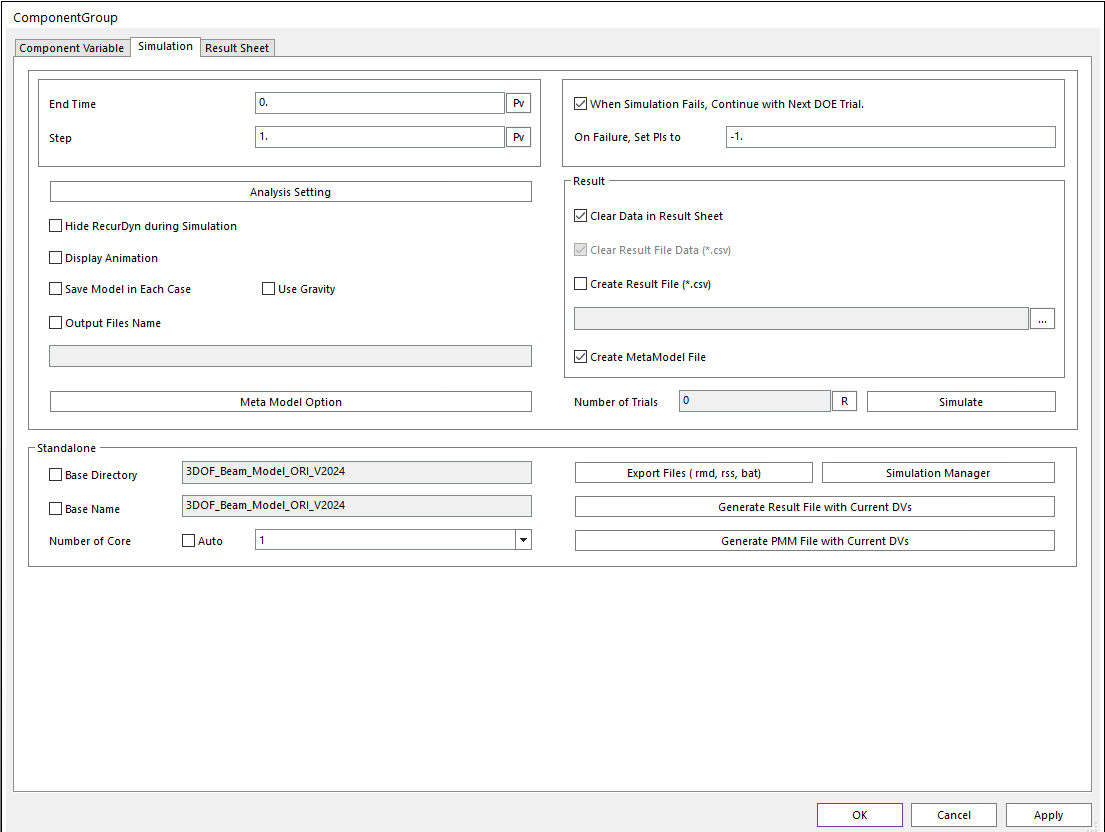
Figure 13.20 Simulation page in ComponentGroup sheet
End Time: Defines the end time of a simulation. If this option is not checked, Report Time Interval option is enabled and End time, Step and Plot Mutiplier Step Factor options are disabled.
Step: Defines the number of sampling data sets that are output for animation.
Analysis Setting: Defines the Static Analysis Parameter.
Hide RecurDyn during Simulation: If this option is checked, the RecurDyn program window is hided during simulation. So, the user can execute the fast analysis. By clicking the right mouse button on the RecurDyn icon at the tray, the user can stop a simulation or activate the RecurDyn main window.
Display Animation: If this option is checked, an animation is displayed during the simulation process.
Save Model in Each Case: Save he each model with used Parametric Value for simulation.
Use Graivty: Set the model using gravity or not.
Output Files Name: Set the output files name.
Meta Model Option: Define meta model option related to multi layer perceptron which iteratively learns (trains) weights (w) and biases (Θ) to minimize the difference (Loss) between the actual function value and the value predicted through the neural network.
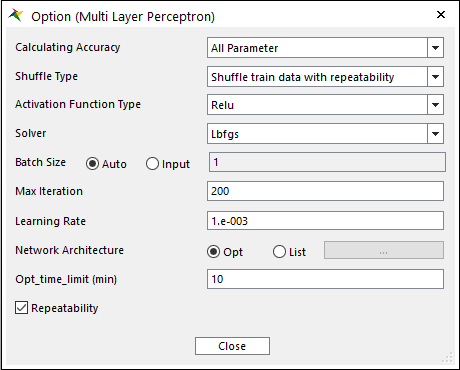
Figure 13.21 Option for Multi Layer Perceptron
Calculating Accuracy: Perform calculation related to the accuracy of the generated meta model. (R2: only R2 value is calculated. All Parameter: R2, PredR2, and CV are calculated)
Shuffle Type: 3 types are supported. (No, Shuffle train data with repeatability, Shuffle train date with repeatability)
Activation Function Type: Define activation function type known as a transfer function used to get the output of node in multi layer perceptron. 4 types are supported. (Identity, Logistic, Tanh, Relu)
Solver: Define optimization technique based on gradient descent method to minimize loss. 4 types are supported. (Lbfgs, Sgd, Adam, Nesterov)
Batch Size: The number of arbitrary training points to be extracted from all training points for loss calculation. (In the case of Auto, it is automatically designated according to the total number of train data.)
Max Iteration: Limitation of the number of iterations for loss calculation.
Learning Rate: Set the degree of training for each iteration. (If set too large, training will not work, if set too small, the convergence speed will be slow.)
Network Architecture: Define the number of hidden layers in the multi layer perceptron and the number of neurons in each hidden layer. If set to Opt, the network architecture is automatically determined through optimization.
Opt_time_limit(min): This option is used when the Network Architecture option is set to Opt, which sets the allowable minutes for Network Architecture optimization.
Repeatability: Define whether random seed is fixed. (creates a model with the same performance every time)
When Simulation Fails, Continue with Next DOE Trial: The simulation does not stop, when simulate fails. And the simulation is continued to the next DOE trial.
On Failure, Set PIs to: Set on the Result Sheet as a performance index’s value when the simulation fails. Only numbers can be inputted.
Clear Data in Result Sheet: Clear result data in result sheet before reporting.
Clear Result File Data: When creating a result table, delete the existing result table.
Create Result File: Create a file containing result table with the set name.
Number of Trials: This is the number of simulations executed based on DOE table and can be updated through the Refresh button.
Simulate: This button proceeds with the analysis as much as the determined Number of Trial.
Note
Static analysis is performed by changing the solver type of RecurDyn to exe solver. Therefore, it cannot be performed by executing two or more RecurDyn.
Standalone: You can perform DOE analysis by using Stand-alone solver.
Base Directory: Root directory of DOE model files.
Base Name: Prefix name of the file related to the created model.
Number of Core: The number of Solver Cores defined in the RMD file can be defined. This value is separate from the value in the Simulation Settings and is applied only when exporting RMD from DOE. Since this value has a great influence on the analysis performance, it is necessary to set it according to the environment.
Export Files (RMD, RSS, BAT): Export RMD and RSS files including PI information. In addition, a batch file that can simulate all models by batch command is created.
Simulation Manager: Utility execution that supports multi-simulation execution. (If base directory is set, automatically add cases). Refer to Simulation Manager.
Generate Result File with Current DVs: Create the result file with rpi information under the base directory. (The RPI file supports only expression type)
Generate PMM File with Current DVs: Create the PMM file with rpi information under the base directory. (The RPI file supports only expression type)
13.2.1.2.3. Result Sheet Page
After finishing component analysis, you can check result table which consist of DOE table and response data of them, and the functions to analyze the result with a chart is also supported.
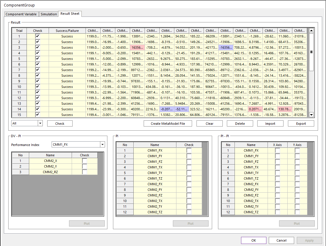
Figure 13.22 Result Sheet page in ComponentGroup sheet
Check: If you select the combo box (All/Failure/Success) and click the check button, only the relevant item is checked.
Clear: Clear the analysis results.
Delet: Delete the checked results.
Import: Import the result table file.
Export: Export the result table file.
DV-PI Plot: Chart of PI(Component Reaction Force) values corresponding to DV(Deformation of each Interface Marker’s DOF) values.
PI Plot: Chart of PI(Component Reaction Force) values.
PI-PI Plot: Chart showing two selected PI(Component Reaction Force) values on the defined axis.
Note