9.1.2. Special Element
These elements do not represent a feature of the structure but play a key role in defining characteristic. For example, the constraints for each node and a specialized lumped mass can be defined.
Rigid Element
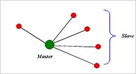
Figure 9.12 Rigid element
Rigid elements are used to define a constraint condition such as a Fixed Joint. A primary node and secondary nodes determine a constraint condition of the element. You can imagine that fixed joints connect the primary node and all of the secondary nodes.
All the secondary nodes degrees of freedom are rigidly linked with the primary node.
There is no limit on the number of secondary nodes.
Interpolation Element
Interpolation elements is a constraint element for the nodes of an FFlex body. This element is similar to what is often called an RBE3 Element in finite element software. It constraints a primary node to a node set of secondary nodes. The constraint requires the primary node to be in the average position of the secondary nodes and it requires the primary node to have an orientation which is the average of the orbits of the secondary nodes around the primary node.
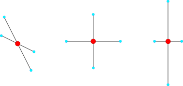
Figure 9.13 The translational constraint of the Interpolation element. The position of the primary node (red) is in the average position of the secondary nodes (blue).
|
|
(a) |
(b) |
(a) The reference configuration of the Interpolation element. (b) The current configuration of the Interpolation element, in which the orientation of the primary node is the average rotation of the secondary nodes around the primary node.
The Interpolation element has some similarities to the constraint-type Rigid element in RecurDyn. Like the Rigid element, it constraints a set of secondary nodes to a primary node. Both the position and the orientation of the primary node is constrained to the positions of the secondary nodes. Note that the orientation of the secondary nodes is not affected by the Interpolation element, which is different from the Rigid element. Furthermore, the Interpolation element allows the secondary nodes to move relative to each other. In contrast, the secondary nodes of the Rigid element move with the primary node like a rigid body.
The Interpolation element was designed for the purpose of providing connections to FFlex bodies that do not stiffen the FFlex mesh around the connection. The Rigid element, which is also often used to make connections to FFlex bodies, causes the FFlex mesh to become stiff around the set of nodes that are constrained by the Rigid element. This is due to the fact that the Rigid element is attempts to lock the nodes together as though they were part of a rigid body. The Interpolation element allows the secondary nodes to move relative to each other, and therefore, the Interpolation element does not stiffen the FFlex mesh around the secondary nodes.
However, the Rigid element is a more general element than the Interpolation element. The Rigid element can be used between a primary node and a single secondary node. The Interpolation element requires that the secondary node set contains at least 4 nodes, and the nodes cannot be co-linear. The constraint-type Rigid element can constrain a primary node to a secondary node in which both nodes have the same coordinates. The Interpolation element requires that the primary node is not in the same location as any of the secondary nodes. In general, the Rigid element is extremely robust and can almost always be used to link a set of nodes to a primary node of an FFlex body. The Interpolation element requires more care when used.
The Interpolation can also be used to distribute forces or torques to a set of nodes. Translational forces applied to a primary node of an Interpolation element is distributed evenly to all of the secondary nodes of an Interpolation element. A torque applied to a primary node of an Interpolation element causes a translational force to be applied to each secondary node that is inversely proportional to the length of the arm between the primary node and the secondary node. In contrast, the Rigid element transmits forces and torques applied to the primary node to the secondary nodes based on the deformation of the body around the secondary nodes.
The Interpolation element is composed of 2 separate constraints.
\({{\mathbf{\Phi }}^{RBE3}}=\left[ \begin{matrix} \mathbf{\Phi }_{trans}^{RBE3} \\ \mathbf{\Phi }_{rot}^{RBE3} \\ \end{matrix} \right]=\mathbf{0}\)
\(\mathbf{\Phi }_{trans}^{RBE3}\) is a translation constraint and \(\mathbf{\Phi }_{rot}^{RBE3}\) is a rotational constraint. \(\mathbf{\Phi }_{trans}^{RBE3}\) and \(\mathbf{\Phi }_{rot}^{RBE3}\) are each composed of 3 equations regardless of the number of secondary nodes used in the constraint. Therefore, each Interpolation element constraint \({{\mathbf{\Phi }}^{RBE3}}\) adds 6 constraint equations to the system of equations of motion.
Translational Constraint
The translational constraint \(\mathbf{\Phi }_{trans}^{RBE3}\) requires that the primary node must be in the average position of the secondary nodes.
\({{\mathbf{q}}^{m}}=\cfrac{1}{n}\sum\limits_{i=1}^{n}{\mathbf{q}_{i}^{s}}\)
where \({{\mathbf{q}}^{m}}\) is the \(3\times 1\) vector of translational coordinates of the primary node, \(n\) is the number of secondary nodes in the Interpolation element, and \(\mathbf{q}_{i}^{s}\) is the \(3\times 1\) vector of translational coordinates of the ith secondary node.
Therefore, the translational constraint is
\(\mathbf{\Phi }_{trans}^{RBE3}={{\mathbf{q}}^{m}}-\cfrac{1}{n}\sum\limits_{i=1}^{n}{\mathbf{q}_{i}^{s}}=\mathbf{0}\)
Rotational Constraint
The rotational constraint of the Interpolation element constraints the orientation of the primary node to the translational position of the secondary nodes. This constraint orients the primary node to minimize its angular difference relative to the secondary nodes. The goal of the rotational constraint of the Interpolation element is to rotate the primary node to follow the rotation of the secondary node set. For example, if the secondary nodes all orbit around the primary node as though they were attached to a rigid body, then the rotational constraint rotates the primary node so that it rotates as though it was also connected to that rigid body. In general, for arbitrary motion of a set of nodes on a flexible body, the nodes might all orbit around the primary node, but they do not orbit as though they are attached to a rigid body. Due to the flexibility of the body, they orbit at slightly different rates. Therefore, the rotational constraint attempts to orient the primary node so that it rotates with the average orbital motion of the node set. This is achieved by using a least square minimization of the difference in direction of the secondary nodes to the primary node in the reference configuration and the current configuration.
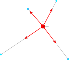
For the rotational constraint, the Interpolation element creates a vector from the primary node to each secondary node in the reference configuration of the nodes of the element.
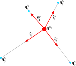
Figure 9.14 One vector is created for each secondary node in the reference configuration.
These vectors are relative to the primary node. If the primary node rotates, these vectors rotate with the primary node.
\(\mathbf{{\hat{v}}}_{i}^{\prime{{r}_{0}}}=\mathbf{A}_{{{m}_{0}}}^{T}\mathbf{\hat{v}}_{i}^{{{r}_{0}}}\)
\(\mathbf{\hat{v}}_{i}^{{{r}_{0}}}={{\left| \mathbf{v}_{i}^{{{r}_{0}}} \right|}^{-1}}\mathbf{v}_{i}^{{{r}_{0}}}\)
\(\mathbf{v}_{i}^{{{r}_{0}}}=\mathbf{q}_{i}^{{{s}_{0}}}-{{\mathbf{q}}^{{{m}_{0}}}}\)
At each time step, the constraint computes the current direction vector from the primary node to each secondary node.
\(\mathbf{\hat{v}}_{i}^{c}={{\left| \mathbf{v}_{i}^{c} \right|}^{-1}}\mathbf{v}_{i}^{c}\)
\(\mathbf{v}_{i}^{c}=\mathbf{q}_{i}^{s}-{{\mathbf{q}}^{m}}\)
There can be some angular difference between the vector to the secondary node in the current configuration and the vector to the secondary node in the reference configuration. The reference vector to a secondary node rotates with the primary node. To find that reference vector in the inertial reference frame, at every time step, the Interpolation element computes
\(\mathbf{\hat{v}}_{i}^{r}={{\mathbf{A}}_{m}}\mathbf{{\hat{v}}}_{i}^{\prime{{r}_{0}}}\)
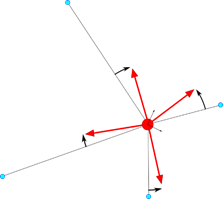
There are generally some angular difference \({{\alpha }_{i}}\) between \(\mathbf{\hat{v}}_{i}^{r}\) and \(\mathbf{\hat{v}}_{i}^{c}\).
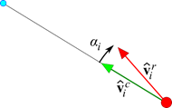
Figure 9.15 The vectors \(\mathbf{\hat{v}}_{i}^{r}\) and \(\mathbf{\hat{v}}_{i}^{c}\) and the angular difference \({{\alpha }_{i}}\) between them. Only 1 secondary node is shown. The primary node is red, the secondary node is blue.
In general, if the secondary nodes all move in some arbitrary direction, it is not possible to orient the primary node so that all reference orientation vectors point directly to each secondary node in the current configuration. There are some difference in direction to some of the nodes. A least square minimization is used to find the orientation of the primary node that minimizes the differences in direction to the secondary nodes.
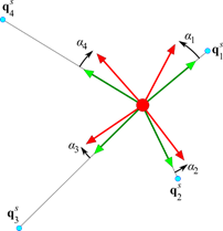
Figure 9.16 The configuration of the primary node such that the sum of the square of the angular differences is minimized.
To create a close approximation to the minimization of the angular differences, a least squares minimization is used. Let \(r\) be the sum of the squares of the sines of the angular differences \({{\alpha }_{i}}\).
\(r=\left[ \sum\limits_{i=1}^{n}{{{\sin }^{2}}{{\alpha }_{i}}} \right]\)
Then \(r\) is a minimum when its derivative with respect to the rotation of the primary node is zero. Since there are 3 independent axes around which the primary node can rotate, 3 minimizations are used. This creates 3 equations of constraint for \(\mathbf{\Phi }_{rot}^{RBE3}\):
\(\mathbf{\Phi }_{rot}^{RBE3}=\left[ \begin{matrix} \cfrac{\partial }{\partial {{\theta }_{x}}}r \\ \cfrac{\partial }{\partial {{\theta }_{y}}}r \\ \cfrac{\partial }{\partial {{\theta }_{z}}}r \\ \end{matrix} \right]=\mathbf{0}\)