9.7.4.3. Plastic
The plastic material in RecurDyn is a J2 plasticity formulation, which is also known as Von-Mises plasticity. This is a small-strain plasticity formulation that is strain-rate independent. It is appropriate for metals at low strain rates. In the elastic range, it is equivalent to the isotropic material. The J2 plastic material in RecurDyn uses an associative flow model.
Plastic materials can be assigned to FFlex bodies that contain hexa-dominant elements (Solid4, Solid5, Solid6 and Solid8) and Shell4 elements.
Plastic materials make to consider the permanent deformation caused by the load over the yield stress. When comparing the elastic materials to the plastic material as shown in Figure 9.72, the different characteristics of plastic material can be shown easily.
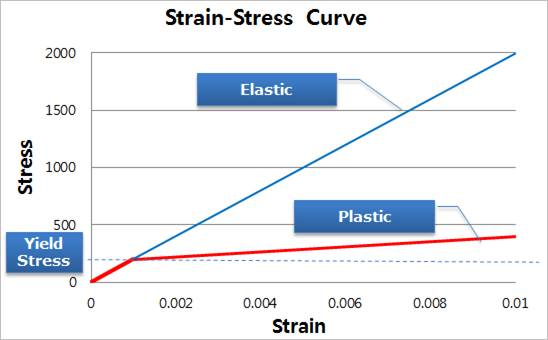
Figure 9.72 Strain vs. stress curves of elastic and plastic materials
Two kinds of work hardening are modeled in RecurDyn’s plastic material: isotropic hardening and kinematic hardening. All plastic materials require isotropic hardening. Optionally, they can also have the kinematic hardening.
3 types for Isotropic Hardening exist:
Multilinear (Default)
Bilinear
Nonlinear
Table 9.9 shows the characteristic of 3 types for Isotropic Hardening of the relationship of strain vs. stress.
 < Multi-linear relationship >
|
 < Bi-linear relationship >
|
 < Non-linear relationship >
|
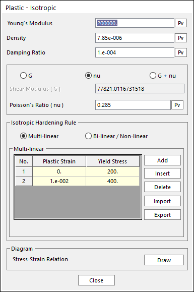
Figure 9.73 Multi-linear isotropic hardening input
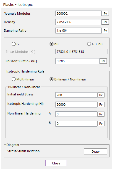
Figure 9.74 Bilinear / Nonlinear isotropic hardening input
The Elastic Properties of the material are defined by the fields.
Young’s Modulus [ \(\text{Force}/\text{Length}^2\) ]
Density [ \(\text{Mass}/\text{Length}^3\) ]
Damping Ratio
Shear Modulus [ \(\text{Force}/\text{Length}^2\) ]
Poisson’s Ratio
The interpretation of these fields is identical to the isotropic elastic material. Please click here for more information on these fields.
Note
When using plastic materials in the analysis, the convergence problem can arise. Especially, RecurDyn’s plastic material is formulated based on J2 plasticity, it is appropriate small-strain problems (for metals) at low strain rates. Therefore, if the slope on the strain-stress curve becomes small rapidly compared to the Young’s Modules, the convergence problem can occur on time integration.
9.7.4.3.1. Hardening
\(f=\left| s-\beta \right|-\sqrt{\frac{2}{3}}Y\le 0\)
- Where,
- \(\mathbf{s}\) is the deviatoric stress.\(Y\) is the yield stress.\(\mathbf{\beta}\) is the back stress.
\(s=2G{{\mathbf{e}}^{e}}=2G(\mathbf{e}-{{\mathbf{e}}^{p}})\)
- Where,
- \(G\) is the shear modulus.\(\mathbf{e}\) is the total deviatoric strain.\({{\mathbf{e}}^{e}}\) is the elastic deviatoric strain.\({{\mathbf{e}}^{p}}\) is the plastic deviatoric strain.
The deviatoric strains satisfy the equation:
\(\mathbf{e}={{\mathbf{e}}^{e}}+{{\mathbf{e}}^{p}}\)
The relationship between the total deviatoric strain \(\mathbf{e}\) and the true strain \(\mathbf{\varepsilon }\) is:
\(\mathbf{e}=\varepsilon -\left( \cfrac{1}{3}\sum\limits_{i=1}^{3}{{{\varepsilon }_{ii}}} \right)\mathbf{I}\)
Where \(\mathbf{\varepsilon }\) is the true strain, measured using small strain theory, and \(\mathbf{I}\) is the 3 \(\times\) 3 identity matrix.
The yield stress \(Y\) implements the isotropic hardening. If the isotropic hardening is present, \(Y\) increase as plastic flow occurs. If no isotropic hardening is present, then \(Y\) is a constant and does not change with plastic flow. The exact form of \(Y\) depends on the type of isotropic hardening that is chosen. In all 3 types of isotropic hardening, \(Y\) is a function of \({{\bar{e}}^{p}}\), where \({{\bar{e}}^{p}}\) is defined by the differential equation:
\({{\dot{\bar{e}}}^{p}}=\gamma \sqrt{\cfrac{2}{3}}\)
Where, \(\gamma =\left\| {{{\mathbf{\dot{e}}}}^{p}} \right\|\)
and for any arbitrary 3 \(\times\) 3 matrix \(\mathbf{M}\):
\(\left\| M \right\|=M:M=\sum\limits_{i,j=1}^{3}{{{m}_{ij}}^{2}}\)
The back stress \(\mathbf{\beta }\) implements the kinematic hardening. It permits the yield surface defined by \(f\) to shift without changing its size. This is easiest to understand with a 1-dimensional example. If uni-axial specimen is stretched, then the kinematic hardening would allow the yield point in tension to rise and simultaneously for the yield point in compression to decrease in magnitude.
In 3-dimensional plastic deformation, the back stress \(\mathbf{\beta }\) allows for the center of the plastic yield surface to shift in the direction of plastic flow.
Isotropic Hardening
Multi-linear Isotropic Hardening: (Default)
The multi-linear hardening is defined by a series of plastic strain/yield stress points.
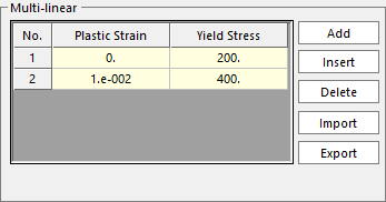
Figure 9.75 The multi-linear point definitions
The points must have ascending values. In other words, for plastic strains \(\varepsilon _{i}^{p}\) and yield stress \(\sigma _{i}^{y}\), where \(i\) indicates the point number:
\(\varepsilon _{i}^{p}<\varepsilon _{i+1}^{p}\) and \(\sigma _{i}^{y}<\sigma _{i+1}^{y}\)
There must be at least 2 points. The first plastic strain value \(\varepsilon _{1}^{p}\) must be zero and the first yield stress \(\sigma _{1}^{y}\) must be greater than zero.
RecurDyn treats the isotropic yield stress (nearly) constant after the multi-linear point. Specifically, RecurDyn treats the isotropic hardening modulus as 1 after the last point defined by the user in the multi-linear table above.
In other words, if the last point defined by the user is \(\varepsilon _{n}^{p}\) and the yield stresses \(\sigma _{n}^{y}\), it is equivalent to RecurDyn automatically defining a final point:
\(\left( \varepsilon _{n+1}^{p},\sigma _{n+1}^{y} \right)=\left( \varepsilon _{n}^{p}+1,\sigma _{n}^{y}+1 \right)\)
if \(\bar{e}_{i}^{p}\le {{\bar{e}}^{p}}\le \bar{e}_{i+1}^{p}\), the yield stress for multi-linear hardening is defined as
\(Y=\sigma _{i}^{y}+H_{i}^{ML}\left( {{{\bar{e}}}^{p}}-\bar{e}_{i}^{p} \right)\)
where, \(H_{i}^{ML}\) is the isotropic hardening modulus of the \(i\) th isotropic hardening segment, which is defined as
\(H_{i}^{ML}=\cfrac{\sigma _{i+1}^{y}-\sigma _{i}^{y}}{\bar{e}_{i+1}^{p}-\bar{e}_{i}^{p}}\)
Multi-linear table buttons:
Add: Add a new plastic strain / yield stress point to the end of the table.
Insert: Insert a new plastic strain / yield stress point into the table below the currently selected row.
Delete: Delete the currently selected row of the table.
Import: Import the data for the table from a text file. Note that the data current data loaded into the table is discarded before importing a file.
Export: Export the table to a text file.
Bilinear Isotropic Hardening:
The bilinear isotropic hardening is defined by only 2 parameters:
Initial Yield Stress (\(\sigma _{initial}^{y}\))
Isotropic Hardening (\({{H}_{i}}\)): the isotropic hardening modulus
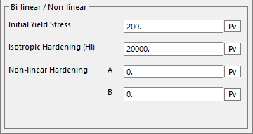
Figure 9.76 Bilinear input fields
The initial yield stress \(\sigma _{initial}^{y}\) and the isotropic hardening modulus must be greater than zero. The yield stress at any time is given by
\(Y=\sigma _{initial}^{y}+{{H}_{i}}{{\bar{e}}^{p}}\)
For the bilinear isotropic hardening, set Nonlinear Hardening fields \(A\) and \(B\) equal to zero.
Nonlinear Isotropic Hardening:
Nonlinear isotropic hardening is defined by 4 parameters:
Initial Yield Stress (\(\sigma _{initial}^{y}\))
Isotropic Hardening (\({{H}_{i}}\)) : the isotropic hardening modulus
\(A\)
\(B\)
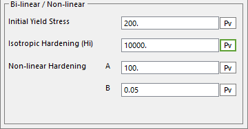
Figure 9.77 Nonlinear input fields
The initial yield stress \(\sigma _{initial}^{y}\) and the nonlinear constants \(A\) and \(B\) must be greater than zero. The isotropic hardening modulus (\({{H}_{i}}\)) must be greater than zero. The yield stress at any time is given by
\(Y=\sigma _{initial}^{y}+{{H}_{i}}{{\bar{e}}^{p}}+A(1-{{e}^{-B{{{\bar{e}}}^{p}}}})\)
Kinematic Hardening
RecurDyn supports only the bilinear kinematic hardening, and therefore, it is defined by only 1 parameter:
Kinematic Hardening (\({{H}_{k}}\)): the kinematic hardening modulus
The linear kinematic hardening is defined by the differential equation:
\(\dot{\beta }=\gamma \cfrac{2}{3}{{H}_{k}}n\)
- Where,
- \(\sum{=}s-\beta\)\(n=\cfrac{\sum{{}}}{\left\| \sum{{}} \right\|}\)
Note that the Kinematic Hardening (\({{H}_{k}}\)) input field is only visible in the plastic material dialog box if Plastic / Isotropic + Kinematic was selected in the Material dialog box.
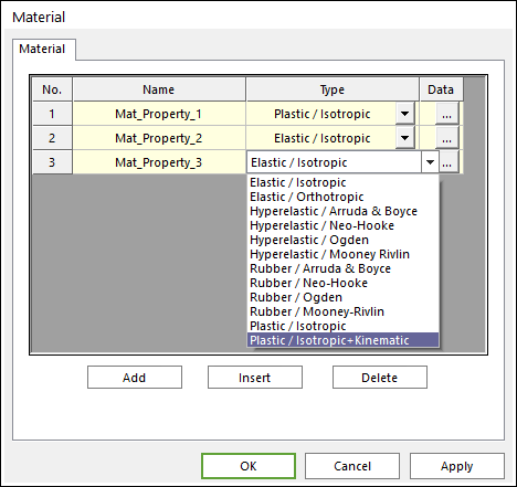
Figure 9.78 Material dialog box
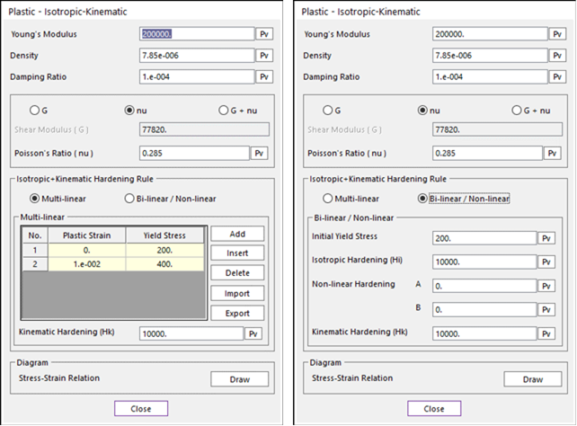
Figure 9.79 Isotropic+Kinematic Hardening input
If Plastic / Isotropic was selected for the material type, then the Kinematic Hardening (\({{H}_{k}}\)) input field is not visible.
9.7.4.3.2. Plotting the Stress-Strain Relationship
The Draw button, as shown in Figure 9.80, in the plastic material dialog box opens the Plastic Hardening Rule plot dialog box containing a plot of the stress-strain relationship defined by the current plastic material input data, as shown in Figure 9.81.
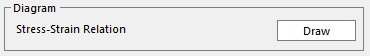
Figure 9.80 The Draw button in the Plastic Material dialog box
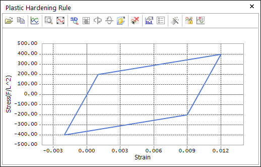
Figure 9.81 The Plastic Hardening Rule plot dialog box
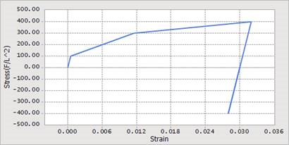
The Plastic Hardening Rule dialog box contains a plot that corresponds to the axial stress versus the total axial strain that would be experienced by a specimen of material subjected to a tension and then a compression load in a uniaxial test. The load magnitude follows a pattern like the one shown in Figure 9.82.
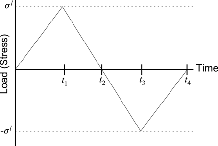
Figure 9.82 Hypothetical axial load applied to a specimen
For the bilinear and nonlinear isotropic hardening (with or without the kinematic hardening), the load \({{\sigma }^{l}}\) is 2x the initial yield stress. In the case of the nonlinear isotropic hardening, though, it is possible that the \({{\sigma }^{l}}=2\sigma _{initial}^{y}\) is unreachable. This occurs when \({{H}_{i}}=0\), \({{H}_{k}}=0\), and \(A\le \sigma _{initial}^{y}\). Therefore, in the case that \({{H}_{i}}=0\) and \({{H}_{k}}=0\), the load \({{\sigma }^{l}}\) that is used is
\({{\sigma }^{l}}=\min (2\sigma _{initial}^{y},0.95\cdot (A+\sigma _{initial}^{y}))\)
In the case of the multi-linear isotropic hardening, the load \({{\sigma }^{l}}\) is chosen so that at time \({{t}_{1}}\), the yield stress is \(Y=\sigma _{n}^{y}\). Note that if the kinematic hardening is used, \(\sigma _{n}^{y}\ne {{\sigma }^{l}}\) because the kinematic hardening introduces a back stress \(\mathbf{\beta }\).
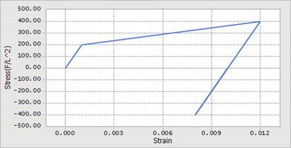
The slope of the total axial strain to axial stress curve during the plastic flow is expected to be
\({{E}_{effective}}=\cfrac{E{{H}_{total}}}{E+{{H}_{total}}}\)
where \({{H}_{total}}\) is the sum of the isotropic hardening modulus and the kinematic hardening modulus.
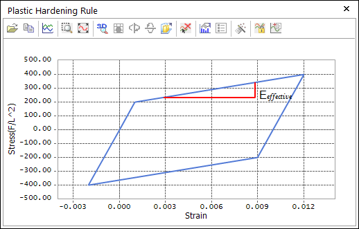
Figure 9.83 The slope of the total strain vs. stress
Simo, J. C., and Hughes, T. J. R., Computational Inelasticity, Springer, 1998