7.2.1.5. Filter
7.2.1.5.1. Definition of Filter Analysis
You can filter curve data to remove or emphasize the specific region of time signal. Two methods are supplied for filtering. One is a transfer function. The other is a Butterworth filer.
Transfer function
Directly specifies the coefficients of transfer function.
Butterworth filter
Computes the coefficients of a transfer function by Butterworth filter algorithm. The Butterworth approximation and bilinear transform are used to obtain transfer function of filter.
Digital Filter
The filter of RecurDyn/Plot is a digital filer. The most general filter takes a sequence \(x_k\) of input points and produces a sequence \(y_n\) of output points by the formula
\(y_n=\sum _{k=0}^{M} {C_k}{x_{n-k}}+\sum _{j=0}^{N-1} {d_j}{y_{n-j-1}}\)
Here the M+1 coefficients \(C_k\) and the N coefficients \(d_j\) are fixed and define the filter response. The filter produces each new output value from the current and M previous input values, and from its own N previous output values. If N=0, so that there is no second sum, then the filter is called nonrecursive or finite impulse response (FIR). If , then it is called recursive or infinite impulse response (IIR).
The relation between the \(C_k\)’s and \(d_j\)’s and the filter response function \(H(f)\) is
where \(\Delta\) is, as usual, the sampling interval.
Taking \(Z\) transform, Transfer function \(H(z)\) is
\(z \equiv e^{2\pi i (f\Delta)}\)
Here \(M\) equals to \(nb\) and \(N-1\) equal to na.
The input-output description of this filtering operation in the Z-transform domain is a rational transfer function,
Design the digital filter
Butterworth approximation
Analog Lowpass Butterworth Filter Design
The magnitude-square response of an N-th order analog lowpass Butterworth filter is given by
\[\begin{flalign} & |H_a(j\Omega)|^2=\frac{1}{1+(\Omega / \Omega_c)^2N} & \end{flalign}\]where \(\Omega_c\) is called the cutoff frequency. The first \(2N-1\) derivatives of \(|H_a(j\Omega)|^2\) at \(\Omega = 0\) are equal to zero. The Butterworth lowpass filter thus is said to have a maximally-flat magnitude at \(\Omega = 0\).
Design of Analog Highpass , Bandpass and Bandstop Filter
RecurDyn/Plot performs the step of the next design process to obtain Highpass , Bandpass and Bandstop Filter.
Step 1 - Develop of specifications of a prototype analog lowpass filter \(H_{LP}(s)\) from specifications of desired analog filter \(H_D(s)\) using a frequency transformation
Step 2 - Design the prototype analog lowpass filter
Step 3 - Determine the transfer function \(H_D(s)\) of desired analog filter by applying the inverse frequency transformation to \(H_{LP}(s)\).
Analog Highpass Butterworth Filter Design
Spectral Transformation of highpass filter is defined as,
\[\begin{flalign} & s=\frac{\Omega_p \hat{\Omega_p}}{\hat{s}} & \end{flalign}\]where, \(\Omega_p\) is the passband edge frequency of \(H_{LP}(s)\) and \(\hat{\Omega}_p\) is the passband edge frequency of \(H_{HP}(\hat{s})\).
Analog Bandpass Butterworth Design Filter
Spectral Transformation of bandpass filter is defined as,
\[\begin{flalign} & s=\Omega_p\frac{\hat{s}^2+\hat{\Omega_0}^2}{\hat{s}(\hat{\Omega_{p2}}-\hat{\Omega_{p1}})} & \end{flalign}\]where, \(\Omega_p\) is the passbandedge frequency of \(H_{LP}(s)\), \(\hat{\Omega}_{p1}\) and \(\hat{\Omega}_{p2}\) are the lower and upper passband edge frequencies of desired bandpass filter \(H_{BP}(\hat{s})\).
Analog Bandstop Butterworth Design Filter
Spectral Transformation of bandstop filter is defined as,
\[\begin{flalign} & s=\Omega_s\frac{\hat{s}^2+\hat{\Omega}}{\hat{s}^2+\hat{\Omega}^2} & \end{flalign}\]where \(\Omega_s\) is the stopband edge frequency of \(H_{LP}(s)\), and \(\hat{\Omega}_{s1}\) and \(\hat{\Omega}_{s2}\) are the lower and upper stopbandedge frequencies of the desired bandstop filter \(H_{BS}(\hat{s})\).
Bilnear Transformation
Bilnear transformation makes digital filter from analog Butterworth filer. The bilinear transformation maps the s domain into the z domain by
\[\begin{flalign} & H(z)=H(s)|_{s=2F_s\frac{s-1}{s+1}} & \end{flalign}\]where, \(F_s\) is the sampling frequency in Herz.
7.2.1.5.2. Property
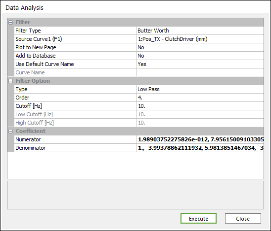
Figure 7.56 Data Analysis dialog box [Filter]
Filter
Filter Type: Selects a type of filter.
Butter Worth
Translator Function
Curve: Selects a curve.
Plot to New Page: If the user wants to draw to a new page, select Yes. If the user wants to draw to the current page, select No. (The default option is No.)
Add to Database: If the user wants to add a desired result to the database, select Yes. (The default option is No.)
Use Default Curve Name: If you want to use the default curve name like “ADD(Acc_TM-Body1(mm/s^2), Vel_TM-Body1(mm/s))”, select Yes. If not, the Chart use the Curve Name.
Curve Name: If Use Default Curve Name is No, Chart use this for a name.
Filter Option
If the user selects Butter Worth Filter, this is activated.
Type: Selects a type.
Low Pass
High Pass
Band Pass
Band Stop
Order
Cutoff(Hz)
Low Cutoff(Hz)
High Cutoff(Hz)
Coefficient
Numerator
Denominator