18.2.2.1. FRF
FRF (Frequency Response Function) is should be needed to simulation in TSG toolkit.
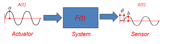
Figure 18.16 A schematic diagram of the TSG model
FRF can be computed like as equation (1) on the frequency domain.
Where, \(\mathbf{A}(s)\) and \(\mathbf{S}(s)\) are Actuator Signal and Sensor Signal on the frequency domain. The \(s\) means a frequency coordinate. The \(\mathbf{F}(s)\) is defined as FRF (Frequency Response Function) in the TSG.
The signals both \(\mathbf{A}(s)\) and \(\mathbf{S}(s)\) are computed using FFT (Fast Furieror Transfom).
After computing FRF, inverse FRF (\({{\mathbf{F}}^{-1}}(s)\)) is computed. Generally, the inverse FRF can be computed by the Pseudo-inverse method.
There are two tabs in FRF dialog box.
FRF tab: There are analysis options to generate FRF.
FRF Result tab: User can check the FRF, the inverse FRF, the actuator signals and the sensor signals.
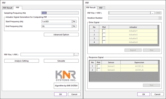
Figure 18.17 FRF dialog box
Step for computing FRF
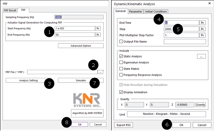
Figure 18.18 Usage FRF simulation
Click FRF icon.
Set Start and End Frequencies.
Click Analysis Setting.
Set the End Time on the Dynamic/Kinematic Analysis dialog. The End Time should be the same of the generated “*.TARGET” file.
Set Step on the Dynamic/Kinematic Analysis dialog. The Step should be the same with (Sampling_Frequency * End_Time).
Click OK to leave the Dynamic/Kinematic Analysis dialog.
Set FRF file name and path on the FRF dialog.
Click Simulation for computing FRF and generating “*.FRF” file.
FRF
All signal entities (Actuator, Sensor and, Target) should be already set to simulate FRF.
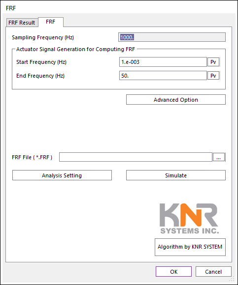
Figure 18.19 FRF dialog box [FRF tab]
Sampling Frequency (Hz): User cannot change this value. This value is the Sampling Frequency (Hz) of loaded “*.TARGET” data.
Actuator Signal Generation for Computing FRF: The Actuator signals (called drive signals) for computing FRF is using a Chirp signal (A sweep function) using following two parameters.
Start Frequency (Hz): Default value is 0.01 Hz.
End Frequency (Hz): Default value is 100.0 Hz.
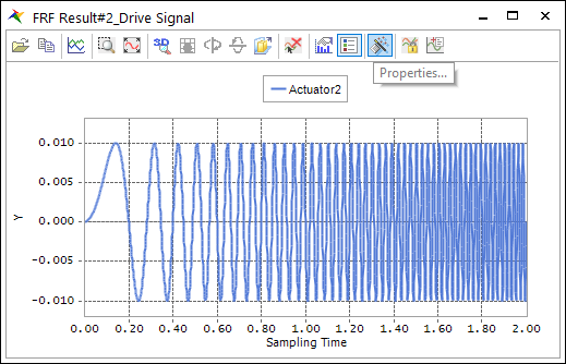
Figure 18.20 Chirp signals
Advanced Option: Currently user can change to magnitude data of each Actuator channels. Default magnitude is set to 1.0.
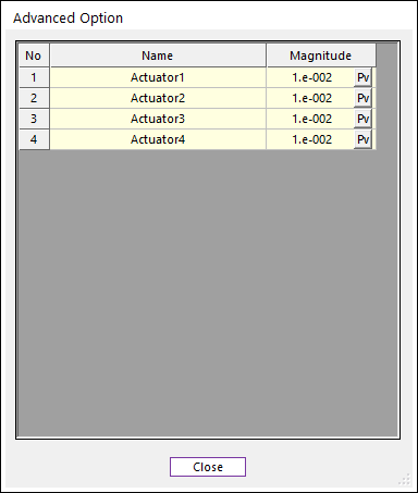
Figure 18.21 Advanced Option dialog box
FRF File (*.FRF): Defines a file name and path by clicking ….
Analysis Setting: Dynamic/Kinematic Analysis dialog is opened. Because, currently TSG is only supported dynamic/kinematic analysis. The End Time and Step should be match on TSG setting.
End Time data on the Dynamic/Kinematic Anlaysis dialog should be the same with the End Time of “*.TARGET” data.
Step data on the Dynamic/Kinematic Anlaysis dialog should be set with (End_Time * Sampling_Frequency).
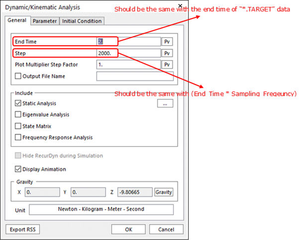
Figure 18.22 Dynamic/Kinematic Analysis dialog
Simulate: Computes FRF and generate “*.FRF” file.
FRF Result
Using this dialog, user can check the FRF, inverse FRF, Actuator signals and, Sensor Signals. In order to check, the “*.FRF” file is needed.
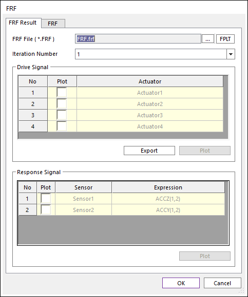
Figure 18.23 FRF dialog box [FRF Result tab]
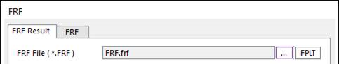
Figure 18.24 FRF File setting
FRF File (*.FRF): Defines “*.FRF” file by clicking ….
FPLT: Checks the FRF and the inverse FRF functions with Plot windows.
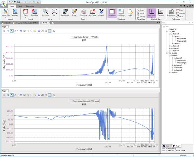
Figure 18.25 Plot view for FRF and Inverse FRF by clicking FPLT
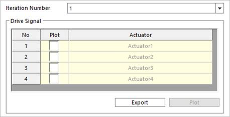
Figure 18.26 Drive Signal region on the FRF Result tab
Iteration Number: Defines the Iteration Number. Iteration Number means the simulation count value for computing FRF. And the Iteration Number is always the same with the number of Actuator channels.
Drive Signal
Plot check box in list view
Export: Generate “*.TAI” file including the Actuator signals on time domain.
Plot: User can see the signal data on the opened scope dialog.
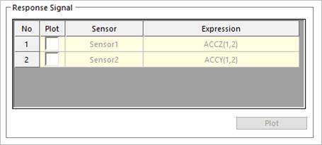
Figure 18.27 Response Signal region on the FRF Result tab
Response Signal
Plot check box in list view
Plot: User can see the signal data on the opened scope dialog.