8.4.3.1. Transient Campbell Diagram Generation Process
There are three steps to create a transient Campbell diagram. The first step is partitioning the data. In this step, you must partition the data against time into a certain number of data frames, each of which becomes a single piece of signal data. During this process, the data in sequential frames may overlap during partitioning. The RPM data is also partitioned using the same signal data against time and the same frames. The second step is to use the FFT algorithm to convert the signal data, which has been partitioned and generated, into a frequency. During this step, you can extract an interaction graph of the frequency and amplitude and define a representative RPM value for each frame. For this, you can use the root mean square (RMS) value or the universal average of each frame. Finally, you can use the FFT data, which is calculated for each frame, and the RPM information to produce a 3D plot.
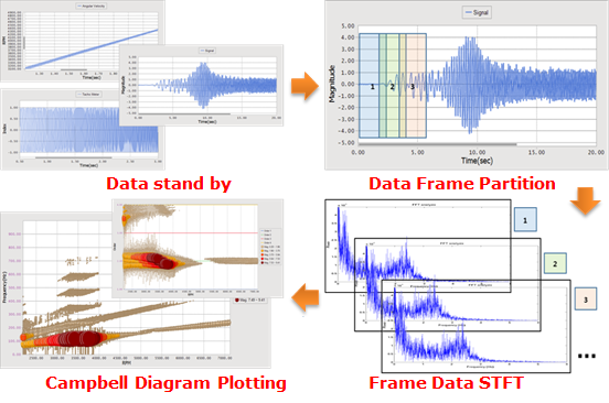
Figure 8.1 Overview of the transient Campbell diagram process
Step 0) Preparing the Data
Plotting a transient Campbell diagram requires the RPM against time value or tachometer data and the time measurement signal. More specifically, RecurDyn’s post-process requires three types of data: time, RPMs, and signal, or time, tacho data, and signal. In this process, the number of data entries for each type of data must be the same.
RPM Data
The RPM data is the system status data that increases or decrease against time. Smaller RPM variations are better.
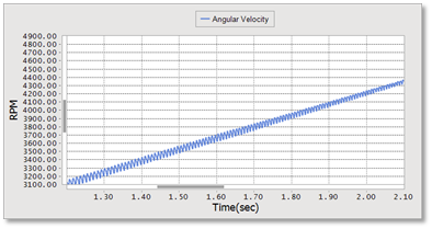
Figure 8.2 RPM data
Tacho Data
The tacho data represents the cyclic trigger signal for the completion of each rotation, in the form of one trigger to one cycle. When this data is inputted in the form of sine function, step function, or impulse function, RecurDyn’s Campbell process must convert it into RPMs before use.
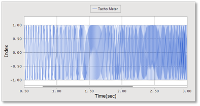
Figure 8.3 Tacho data
Translating tacho data into RPM data
There are several ways to represent the tacho data: peak pulse, step pulse, offset step pulse, sine wave, etc.
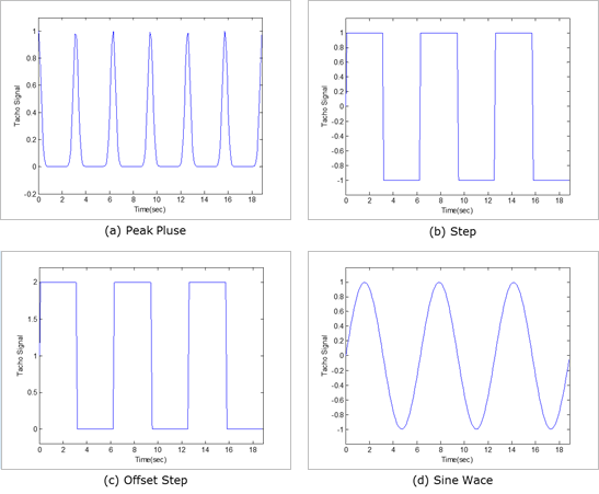
Figure 8.4 Various representations of tacho data
To calculate the correct RPM for each signal type, perform the following steps:
Calculate the RMS of the tacho data.
Tacho data (n) = Tacho data (n) – RMS.
Extract the phase change data point (PCDP) (- to +).
Calculate the RPMs from the delta time.
To calculate the RPM value for one point, calculate the average of the RPM values from the time data for the previous PCDP and the next PCDP.
Finally, use linear interpolation of the calculated RPM values to determine the RPM values of the remaining data points.
The time data remains the same when the tacho signal is converted into the RPM data. After the data conversion, the process is the same as for the RPM data.
Signal Data
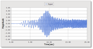
About the tacho data and the RPM data: To measure the RPMs of a system during a test or simulation, the user should measure the speed and tachometer reading. When the user measures only the RPMs, the RPM value may also include high-frequency noise transmitted from the system. Therefore, the noise may influence the calculation of the RPM value for each frame. If the RPM response over time is relatively non-linear, then the influence of this noise may be even more pronounced. In contrast to this, the tacho data only measures the cycle for one rotation, so it automatically eliminates any influence from high-frequency noise. Therefore, it is better to use a sine or step function and produce the tacho data for a periodic function than to measure and use the RPM value.
Step 1) Partitioning Data for STFT (Short Time Fourier Transform)
During this step, the user partitions the signal data while allowing a certain amount of overlap between the partitions. The overlapping frames and data counts are integers and relate to the data counts for the FFT. The formula is as follows.
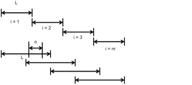
\(T=(n_f-1)\cdot (L-o)+L=n_fL-n_fo+o=d \cdot (n_f-1)+L (d=L-o)\)
\(o=\lambda L (where,0<\lambda<1)\)
- where,
- \(T\) : Total time\(L\): Time of frame data\(Nf\): Fame count for STFT\(o\): Overlap time\(\lambda\): Overlap ratio
The data count is an integer and each frame represent the count of the input data for the FFT (e.g. 256, 512, 1024…). Therefore, in order to use the existing data without using the interpolation to conduct STFT, the user should first select the data count of the frame to minimize the residual data and then determine L and O that can produce proper resolutions. The formula for residual data is as follows.
\(ip_{res}=ip_r-((n_f-1)ip_d+ip_L)\)
where, \(ip_d=ip_L-ip_o\)
\(ip_T\): Total data count\(ip_{res}\): Residual data count\(n_f\): Frame count\(ip_L\): 1 Frame data count\(ip_o\): Overlap data count
After the user determines \(n_f\) and \(ip_L/ip_o\), the user is ready to conduct STFT.
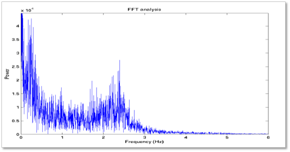
Step 2) Frame Data FFT (fast Fourier transfer)
The user can conduct the FFT for each data frame partitioned in step 1. The basic principles and calculation methods of the FFT are widely known. RecurDyn uses an algorithm from Numerical Recipes (NR) to calculate the data for the Campbell diagram. The signal process does not include interpolation or extrapolation, so the system uses the current signal data. You can use multiple windows to conduct FFT. To extract the magnitude, you can use the amplitude and the PS (power spectrum) or the PSD (power spectrum density).
Step 3) Plotting the Campbell Diagram
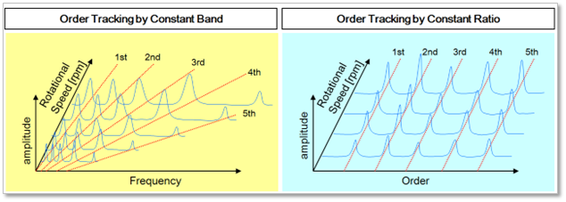
There are many ways to plot the Campbell diagrams, but the Waterfall diagrams are the most popular for the rotor systems. This type of diagram expresses the FFT data in a 3D space. Each point in the 3D space is mapped based on the RPM, frequency, and amplitude values inputted into the algorithm. Some Waterfall diagrams express amplitude through the size of each point in a 2D graph (RPM - Frequency). The user can also use the constant band method or the constant ratio method to draw the Waterfall diagrams.
Order tracking by constant band: Draws the diagram based on the rotational speed and frequency.
Order tracking by constant ratio: Draws the diagram based on the rotational speed and order.