14.3.3. Stress Life Criteria

Manson-Coffin

If the stress level is generally very low and the number of cycles to failure is generally very high, the Manson-Coffin stress life equation is typically used for the high cycle fatigue such as the material fatigue due to the vibration of the structure.

The Manson-Coffin stress life equation of S-N Curve can be written as

\(\frac{\Delta \sigma }{2}={{{\sigma }'}_{f}}{{\left( 2{{N}_{f}} \right)}^{b}}\)

where,

\(\frac{\Delta \sigma }{2}\) ∶ Normal stress amplitude for a cycle

\({{{\sigma }'}_{f}}\) ∶ Fatigue strength coefficient

\(2{{N}_{f}}\) ∶ Reversals to failure

\(b\) ∶ Fatigue strength exponent (material property)

In this life equation, only the stress amplitude is taken into account.

ASME

The ASME life criterion is based on the American Society of Mechanical Engineers (ASME) Boiler and Pressure Vessel code. This code uses the percent reduction in area (RA) as its principal variable.

The ASME equation is solved for the number of cycles to failure.

This equation is shown below.

\(\frac{\Delta \sigma }{2}=\frac{E}{4\sqrt{{{N}_{f}}}}\ln \left( \frac{100}{100-RA} \right)+0.01{{S}_{u}}\times RA\)

where,

\(\frac{\Delta \sigma }{2}\) : Maximum principal stress amplitude (1/2 range)

\(E\) : Elastic modulus (Young’s Modulus)

\({{N}_{f}}\) : Number of Cycles to fatigue

\(RA\) : Percent reduction in area

\({{S}_{u}}\) : Ultimate tensile strength

BWI

The BWI Weld stress life is based on the British Welding Institute’s formulation, which uses the weld class as the basis for the fatigue life estimate while it does not use the material properties.

This method predicts fatigue failure in welded joints. The criterion takes into account local stress concentration which may be due to the weld itself.

The weld equation is solved for cycles to failure. This equation is shown below.

\({{\log }_{10}}\left( {{N}_{f}} \right)={{\log }_{10}}\left( a \right)-d\times stdev+m\times {{\log }_{10}}\left( \Delta \sigma \right)\)

where,

\({{N}_{f}}\) : the number of Cycles to fatigue

\(a\) : the ultimate tensile strength

\(d\) : the constant value

\(m\) : the number of standard deviations below the mean value.

\(stdev\) :the standard deviation of log(\(Nf\)).

The fatigue life estimate is based on the weld class you select. RecurDyn/Durability provides damage life evaluations of Class B/C/D/E/F/F2/G/W/S/T.

Parameters \(a\) and \(m\) are dependent on the weld class.

Mean Stress Effect

The most basic fatigue data are collected in the laboratory by means of testing procedures which employ fully reversed loading, i.e. zero as a stress load cycle. However, the most realistic service situations involve non-zero as stresses. Therefore, it is very important to know the influence that the mean stress has on the fatigue process, so that the fully reversed laboratory data can be employed in the assessment of real situations.

Fatigue data collected from a series of tests designed to investigate different combinations of stress amplitude and mean stress are characterized Figure 14.51 for a given number of cycles to failure. The diagram plots the mean stress with both tensile and compressive along the x-axis, and the alternating constant stress amplitude along the y-axis. This kind of representation was first proposed by Haigh and is therefore commonly referred to as the Haigh diagram.

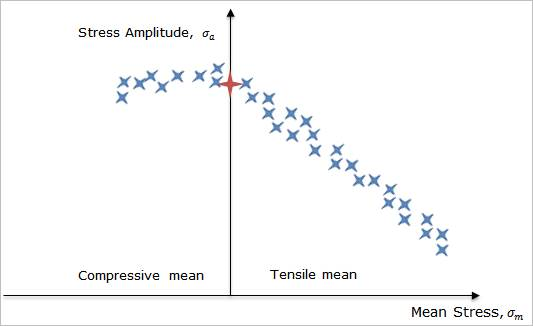
Figure 14.51 Haigh Diagram with fatigue data

The stress amplitude at zero mean stress (\({{S}_{e}}\)) corresponds to the stress amplitude at N cycles to failure as measured by the fully-reversed fatigue test. The failure data points tend to follow a curve which is extrapolated would pass through the ultimate tensile strength (\({{S}_{u}}\)) on the mean stress axis. Notice that the influence of mean stress is different for compressive and tensile mean stress values. Failure appears to be more sensitive to tensile mean stress, than compressive mean stress.

This is called Goodman method. And other methods are offered to update the stress amplitude used for stress-based life equations. The relations on each correction methods are as follows:

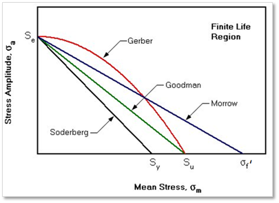
Figure 14.52 Comparison of four correction methods for mean stress effect

Goodman: \(\frac{{{\sigma }_{a}}}{{{S}_{e}}}+\frac{{{\sigma }_{m}}}{{{S}_{u}}}=1\)

Gerber: \(\frac{{{\sigma }_{a}}}{{{S}_{e}}}+{{\left( \frac{{{\sigma }_{m}}}{{{S}_{u}}} \right)}^{2}}=1\)

Soderberg: \(\frac{{{\sigma }_{a}}}{{{S}_{e}}}+\frac{{{\sigma }_{m}}}{{{S}_{y}}}=1\)

Morrow: \(\frac{{{\sigma }_{a}}}{{{S}_{e}}}+\frac{{{\sigma }_{m}}}{{{\sigma }_{f}}^{'}}=1\)

where,

\({{S}_{e}}\): Effective alternating stress at failure for a life time of N_f cycles

\({{S}_{u}}\): Ultimate strength

\({{S}_{y}}\): Yield strength

\({{\sigma }_{f}}'\): Fatigue strength coefficient

\({{\sigma }_{m}}\): Mean normal stress for a cycle

Therefore, there are four types for representing the mathematical relationship such as Goodman, Gerber, Soderberg and Morrow as shown Figure 14.52.