21.4.6.2. RIA Method based on Sequential Approximate Optimization (SAO) Approach
In reliability analysis, when a performance function or a limit state function \(g(X)\) is defined as the random variable vector, \(X=\{{{x}_{1}},{{x}_{2}},...,{{x}_{n}}\}\), the limit state function can divide the design region into safe and failure regions along the boundary \(g(X)=0\). Then, the probability of failure for a system is
\({{p}_{f}}=\int_{\Omega }^{{}}{{{f}_{x}}(x)dx}\)
In which \({{f}_{x}}\) is a joint probability density function for \(x\) and \(\Omega\) is failure region. As explained in the Monte Carlo simulation chapter has been widely used to avoid the above multiple integration. It requires, however, too many simulations. Thus, in this section, another approach is explained to estimate the probability of failure, which is based on the uncorrelated standard normal variable space.
21.4.6.2.1. Equivalent Normal Concepts
Suppose that the statistical distribution for random variable vector, \(X=\{{{x}_{1}},{{x}_{2}},...,{{x}_{n}}\}\) is known. Then, the component \({{x}_{i}}\) is dependent and continuous for the probability density function \({{f}_{x}}(X)\) and the probability distribution function \({{F}_{x}}(X)\). Also, it is assumed that the limit state function
\(Z=g(X)\)
is a continuous function of \(X\). Then, let’s define the probability of failure as
\({{p}_{f}}=\Pr ob[g(X)<0]\)
When the limit state function is linear, the probability of failure can be exactly evaluated without the multiple integrations. For all random variables \({{x}_{i}}\), let’s consider that the mean value are \({{\mu }_{i}}\) and the standard deviation are \({{\sigma }_{i}}\). Then, the normalized variable \({{u}_{i}}\) is defined by
\({{u}_{i}}=\frac{{{x}_{i}}-{{\mu }_{i}}}{{{\sigma }_{i}}}\)
The probability of failure is given by
\({{p}_{f}}=\Phi (-\beta )\)
where \(\Phi\) is ‘standard normal distribution function’ and the safety factor \(\beta\) can be calculated from the geometric relation shown in Figure 21.154. The safety factor \(\beta\) can be called as Reliability Index. Suppose that the linear limit state function is \(Z=R-S\). Also, it is assumed that \(R\) and \(S\) are normal distributions. Then, the reliability index is denoted as
\(\beta =\frac{{{\mu }_{z}}}{{{\sigma }_{z}}}=\frac{{{\mu }_{R}}-{{\mu }_{S}}}{\sqrt{{{\sigma }_{R}}^{2}+{{\sigma }_{S}}^{2}}}\)
which is referred to as FOSM (First-Order Second Moment) method or MVFOSM (Mean Value First-Order Second-Moment) method.
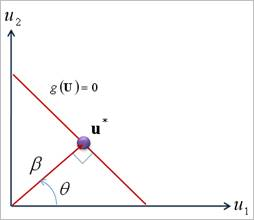
Figure 21.154 The Safety Index for Linear Limit State Function
In order to extend the above concept to the general probabilistic distribution, the equivalent normalization concept is introduced. This uses transformation matrix to change the random variables into the equivalently normalized variables.
\(u=T(x)\) or \(x={{T}^{-1}}(u)\)
where \(T(x)\) depends on the distribution of \(x\). In the standard normal variable space shown in Figure 21.154, the probabilistic density function is decreased exponentially from the origin. Thus, the probability of failure \((\Phi (-\beta ))\) can be easily evaluated by obtaining the minimum distance(\(\beta\)) from the origin to the tangent plane of limit state function, which is graphically explained in Figure 21.155.
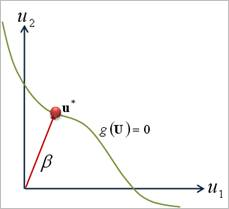
Figure 21.155 Graphical Representation of Reliability Index Analysis (RIA)
21.4.6.2.2. First-Order Reliability Method (FORM)
The mathematical formulation, for Reliability Index Analysis(RIA), is simplified to find the minimum distance to the limit state function in the standard normal variable space.
\(\underset{u}{\mathop{\min }}\,\beta =\left\| {{u}^{T}}u \right\|\)
subject to
\(g(u)=0\)
This formulation is developed by Hasofer and Lind, which has been referred to as AFOSM ( Advanced First - Order Second Moment) method that overcomes the lack of invariance of MVFOSM.
There are many algorithms available that can solve this problem, such as mathematical optimization methods or other iteration algorithms. In the literature, several constrained optimization methods are used to solve the problem directly, which include primal optimization methods (Method of Feasible Directions, Gradient Projection and Generalized Reduced Gradient) and transformation methods (Penalty Function and Augmented Lagrange Multiplier). Each method has its advantages and disadvantages, depending upon the characteristic of the algorithm and the nature of the problem.
Unlike the optimization methods, another approach is the iteration algorithm. The currently used iteration method is HL-RF (Hasofer, Lind, Rackwits and Fiessler) method, which was originally proposed by Hasofer and Lind for second-moment reliability analysis and later extended by Rackwitz and Fiessler to include random variable distribution information.
The HL-RF method approximates the hyper-surface \(Z=g(U)\) by its tangent plane \(\tilde{Z}=g({{U}^{k}})+\nabla g({{U}^{k}})(U-{{U}^{k}})=0\) at the most probable point (MPP):math:{{U}^{k}}, and then an improved point \({{U}^{k+1}}\) is obtained by computing the shortest distance from the approximate hyper-surface \(\tilde{Z}\) to the origin. The recurrence formula for \({{U}^{k+1}}\) is expressed as follows:
\({{U}^{k+1}}=\frac{1}{{{[\nabla g({{U}^{k}})]}^{2}}}\left[ \left\lfloor \nabla g({{U}^{k}}) \right\rfloor {{U}^{k}}-g({{U}^{k}}) \right]\nabla g{{({{U}^{k}})}^{T}}\)
When \(g(U)\) is nonlinear function, the iterative solution \({{U}^{k+1}}\) is only approximate. Thus, the above formula is applied repeatedly until the sequence \({{U}^{k}}\) converges to the minimum distance point. The HL-RF method has the advantage over the optimization methods in that it is simple and faster. However, this method does not guarantee the global convergence.
Recently, in order to reduce the computational burden of the mathematical optimization method, the sequential approximate optimization (SAO) method has been applied to solve the original RIA problem, which solved the following approximate optimization problem until the sequence \({{U}^{k}}\) converges to the minimum distance point.
\(\underset{u}{\mathop{\min }}\,\beta =\left\| {{u}^{T}}u \right\|\)
subject to
\(\tilde{g}(u)=0\)
in which the limit state function is approximate by using the gradient information and function information. When the gradient information is available, two-point methods, widely used in structural optimization, are widely used. Otherwise, the meta-modeling methods including RSM are newly tried.
21.4.6.2.3. Second-Order Reliability Method (SORM)
When FORM applies to the limit state functions with same MPP, their failure probabilities are estimated as equal values. Figure 21.156 shows the linear and the nonlinear limit state functions with same MPP. But it is apparent that the failure probability of nonlinear limit state function(\({{g}_{n}}\)) should be less than that of the linear limit state function (\({{g}_{i}}\)). In Figure 21.156, the shade areas are the failure regions, respectively.
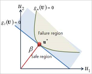
Figure 21.156 Linear and Nonlinear Limit State with sample MPP
The curvature of the nonlinear limit state function is ignored in the FORM approach, which uses only a first-order approximation at MPFP. Thus, the second-order reliability method (SORM) was widely studied to include the curvature information. The SORM analysis requires a second-order polynomial:
\({{G}_{2}}(u)\approx {{a}_{0}}+\sum\limits_{i=1}^{N}{{{a}_{i}}({{u}_{i}}-u_{i}^{*})+}\sum\limits_{i=0}^{N}{{{b}_{i}}{{({{u}_{i}}-u_{i}^{*})}^{2}}+\sum\limits_{i=1}^{N}{\sum\limits_{j=1}^{i-1}{{{c}_{ij}}({{u}_{i}}-u_{i}^{*})({{u}_{j}}-u_{j}^{*})}}}\)
This definition requires \(N(N-1)/2\) second order derivatives. Breitung derived the following asymptotic formula for large
\({{p}_{f}}\approx \Phi (-\beta )\prod\limits_{i=1}^{N-1}{{{(1-\beta {{k}_{i}})}^{-1/2}}}\)
where \({{k}_{i}}\) are the principal curvatures at the most probable failure point. Although SORM could improve the accuracy, it may become expensive if a large number of costly numerical analyses, such as large-scale CAE analyses embedded in the limit state functions, are involved.
21.4.6.2.4. Dimension Reduction Method (DRM)
Recently, the univariate dimension reduction methods (DRM) are newly presented, which can solve highly nonlinear reliability problems more accurately or more efficiently than FORM/SORM and Monte Carlo simulation methods. A major advantage of these decomposition methods so far based on the mean value points or MPP as reference points, over FORM/SORM is that higher-order approximations of performance functions can be achieved using function values only.
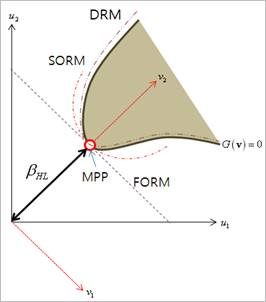
Figure 21.157 Limit Function Approximations by Various Methods
The transformed limit state functions \(g(u)=0\) and \(G(v)=0\) are the maps of the original limit state function \(g(x)=0\) in the standard Gaussian space (u space) and the rotated Gaussian space (v space), respectively, as shown in Figure 21.157. The nearest point on the limit-state surface to the origin, denoted by the MPP (\({{u}^{*}}\) or \({{v}^{*}}\)) or beta point, has a distance \({{\beta }_{HL}}\), which is commonly referred to as the Hasofer-Lind reliability index. The determination of MPP and \({{\beta }_{HL}}\) involves, based on FORM, standard nonlinear constrained optimization and is usually performed in the standard Gaussian space.
Consider a univariate approximation of \(G(v)\), denoted by
\({{\tilde{G}}_{l}}(v)\equiv {{\tilde{G}}_{1}}({{v}_{1}},{{v}_{2}},...,{{v}_{N}})=\sum\limits_{i=1}^{N}{G(v_{1}^{*},...,v_{i-1}^{*},v_{i}^{*},v_{i+1}^{*},...,v_{N}^{*})-(N-1)G({{v}^{*}})}\)
where each term in the summation is a function of only one variable. As higher-order univariate terms can be included in the approximation, the univariate approximation may be more accurate than FORM and SORM. In addition to the MPFP as the chosen reference point, the accuracy of the univariate approximation may depend on the orientation of the first \(N-1\) axes. In general, a Gram-Schmidt orthogonalization is used to determine the transformation matrix.
Finally, the failure probability is approximated by
\({{p}_{f}}=\Pr ob[G(v)<0]\cong \Pr ob[{{\tilde{G}}_{l}}(v)<0]\)
The univariate integration can be evaluated easily by standard one-dimensional Gauss-Hermite numerical quadrature. The decomposition method involving univariate approximation and univariate integration is referred to as the MPP-based Dimension Reduction Method (MPP-based DRM).
21.4.6.2.5. Example for Normal Distributions
Let’s reconsider the example problem explained in the Example for Normal Distributions of Monte Carlo Simulation. The performance function of a mechanical system is given by
\(z=g({{x}_{1}},{{x}_{2}})=x_{1}^{2}+x_{2}^{2}=18\)
Where \({{x}_{1}}\) and \({{x}_{2}}\) are the random variables with normal distributions. Their mean values and standard deviation values are (10,10) and (5,5), respectively. If the performance function \(Z>0\), then the system is always safe. Find the probability of failure for the mechanical system.
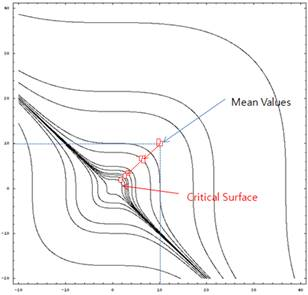
Figure 21.158 The convergence trajectory by AFORM in AutoReliability
Sol: Numerical optimization approach of AutoReliability provides three methods such as AFORM, AFORM+DRM1, and AFORM+DRM2. All methods are based on Meta-model based SAO, which uses similar concept of AutoDesign. The sequence, however, is more efficient than that of AutoDesign because the design problem for reliability analysis is only one formulation unlike the general optimization.
Figure 21.158 shows the convergence trajectory of AFORM (Advanced First - Order Reliability Method) which solve the reliability index analysis problem by using meta-model based SAO. It requires only 17 evaluations until converged. Among them, 13 evaluations, sampled from discrete Latin Hypercube design, are used to construct the initial meta-model. The remaining 4 points are used to validate the results obtained in the SAO steps. The most probable failure point is (1.9897, 2.1632). The probability of failure is 0.01250 and the reliability index is 2.2412.
Next, AFORM+DRM-1 employs the MPFP based DRM. This method employs the numerical integration for the meta-model at MPFP. Thus, it does not require additional evaluation than AFORM. Thus, it requires only 10 evaluations. The estimated failure probability and the reliability index are 0.006689 and 2.4745, respectively.
Finally, Figure 21.159 shows the convergence trajectory by AFORM+DRM2. Unlike AFORM+DRM-1, this method samples the exact evaluations when the numerical integration at MPFP. The 5-point gauss integration is used. Thus, it requires the additional evaluations such as 4*(NDV-1) points. Thus, it requires 14 points (10 evaluations for AFORM and 4 evaluations for integration). The estimated failure probability and the reliability index are 0.00666 and 2.4745, respectively. These values are exactly equal to that of AFORM+DRM1, which represents the meta-model is nearly exact about MPFP.
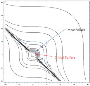
Figure 21.159 The convergence trajectory by AFORM+DRM2 in AutoReliability
Comparing with the results of Monte-Carlo simulation shown in the Figure 21.151, the probability of failure (\({{p}_{f}}=0.0067\)) of the SAO based approach is nearly equal to that of Monte-Carlo 5000 simulations (\({{p}_{f}}=0.0068\)). However, it is noted that AFORM+DRM1 and AFORM+DRM2 used only 17 and 21 evaluations, respectively.
21.4.6.2.6. Design Sensitivity Analysis of Reliability Index
As a final discussion, let’s consider the method of estimating the what-if effect that some change in problem parameters such as mean and standard deviation values has on the most probable failure point (MPP). Suppose that the mean value of loads or the standard deviations of random design variables are changed after we have already found an MPFP. Then, we want to estimate the effect that this has on the reliability analysis without actually solving the reliability analysis problem over again.
Reconsider the following reliability analysis formulation described in First-Order Reliability Method (FORM).
\(\underset{u}{\mathop{\min }}\,\beta =\left\| {{u}^{T}}u \right\|\)
subject to
\(g(u)=0\)
This problem is an optimization problem. Thus, an optimum \({{u}^{*}}\) should satisfy the following Kuhn-Tucker optimality conditions.
\({{\nabla }_{u}}L(u,\lambda )={{\nabla }_{u}}\beta ({{u}^{*}})+\lambda {{\nabla }_{u}}g({{u}^{*}})=0\)
\({{\nabla }_{\lambda }}L(u,\lambda )=g({{u}^{*}})=0\)
Now, the variation form of the objective is
\(\delta \beta =\underset{u}{\mathop{\min }}\,{{\nabla }_{u}}\beta ({{u}^{*}})\delta u\)
Then, the design sensitivity values of Reliability Index can be represented as
Finally, in order to satisfy the Kuhn-Tucker optimality conditions, it can be simplified as
where Lagrange multiplier can be determined as
from the optimality conditions. The design sensitivity for the failure property can be determined as
Let’s reconsider the example explained in Example for Normal Distributions. The reliability analysis was performed at mean values (10, 10) and standard deviations (5, 5). If the mean values are increased, then is the reliability index increased or decreased? Or if the standard deviations are decreased, is the failure probability decreased or increased?
We can know this information from design sensitivity analysis. AutoReliability provides the analytical design sensitivity results. Table 21.13 lists the design sensitivity results.
AFORM |
AFORM+DRM2 |
|
\(d\beta /d{{\mu }_{1}}\) |
0.1414 |
0.1280 |
\(d\beta /d{{\mu }_{2}}\) |
0.1414 |
0.1280 |
\(d\beta /d{{\sigma }_{1}}\) |
-0.2240 |
-0.2028 |
\(d\beta /d{{\sigma }_{2}}\) |
-0.2240 |
-0.2028 |
\(d{{p}_{f}}/d{{\mu }_{1}}\) |
-0.004589 |
-0.002397 |
\(d{{p}_{f}}/d{{\mu }_{2}}\) |
-0.004589 |
-0.002397 |
\(d{{p}_{f}}/d{{\sigma }_{1}}\) |
0.007270 |
0.003798 |
\(d{{p}_{f}}/d{{\sigma }_{2}}\) |
0.007270 |
0.003798 |
In the above table, AFORM and AFORM+DRM2 give same signs but different values of design sensitivity. Why? It is because they give different reliability index values(\(\beta\)). Thus, AutoReliability modifies the design sensitivity values to the degree of difference of reliability index value.
From the design sensitivity analysis results, we can know that the failure probability can be decreased when two mean values are increased. If the standard deviations are increased, the failure probability can be increased.
This information can be verified from the figure. When two mean values are increased, the current point is moved away from MPP. This represents that the current point is moved into safer region.
Next, consider the Monte Carlo simulation. If the standard deviations are increased, the sample points are more scattered from the current point. Thus, the number of failure points can be increased. Thus, the failure probability can be increased.
Reference
Achintya Haldar and Sankaran Mahadevan, Probability, Reliability, and Statistical Methods in Engineering Design, John Wiley & Sons, Inc., New York, 2000.
Singiresu S. Rao, Reliability-Based Design, McGraw-Hill, Inc., New York, 1992.
Hasofer, A.M. and Lind, N.C., “Exact and invariant second-moment code format”, J. Engng. Mech. Div. ASCE, 100(EMI), pp. 111-121, 1974.
Rackwitz, R. and Fiessler, B., “Structural reliability under combined load sequence”, Comput. Struct., Vol. 9, pp. 489-494, 1978.
Wang, L. and Grandhi, R.V., “Effivient Safety Index Calculation for Structural Reliability Analysis”, Computer & Structures Vol. 52, No.1, pp. 103-111, 1994.
Der Kiureghian, A. and Dakessian, T., “Multiple design points in first and second-order reliability”, Structural Safety, Vol. 20, No.1, pp.37-49, 1998.
Breitung, K., “Asymptotic Approximations for Multinormal Integrals”, Journal of Engineering Mechanics, ASCE, Vol. 110, No. 3, pp. 357-366, 1984
Wei, D. and Rahman, S., D.,”Structural reliability analysis by univariate decomposition and numerical integration”, Probabilistic Engineering Mechanics, Vol. 22, pp. 27-38, 2007.
Rahman, S. and Xu, H., “A univariate dimension-reduction method for multi-dimensional integration in stochastic mechanics”, Probabilistic Engineering Mechanics, Vol. 19, pp. 394-408, 2004.
Rahman, S. and Wei, D.,”A univariate approximation at most probable point for higher-order reliability analysis”, Int. J. of Solids and Structures, Vol. 43, pp. 2820-2839, 2006.
Min-Soo Kim, User’s Guide for PV-INOPL: Meta-Model based Reliability Index Analysis, Institute of Design Optimization Inc., Korea, 2009.