5.5. Frequency Response Analysis
Frequency Response Analysis is a measure of magnitude and phase of the output as a function of frequency, in comparison to the input. In simplest terms, if a sine wave is applied into a system at a given frequency, a linear system responds at the same frequency with a certain magnitude and a certain phase angle relative to the input.
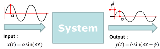
Figure 5.28 Frequency Response Analysis
Where, the magnitude and phase angle are calculated as following.
State matrix is needed for performing Frequency Response Analysis. Definition of the State Matrix is as follows.
\(\begin{aligned} & \mathbf{\dot{x}}=\mathbf{Ax}+\mathbf{Bu} \\ & \mathbf{y}=\mathbf{Cx}+\mathbf{Du} \\ \end{aligned}\)
Where, A, B, C, and D are State matrix of a system including MBD and RFlex.
\(\mathbf{x}\) is generalized coordinates defined as \(\mathbf{x}\equiv \left\{ \begin{matrix} {\mathbf{\dot{q}}} \\ \mathbf{q} \\ \end{matrix} \right\}\).
\(\mathbf{u}\) and \(\mathbf{y}\) are Input and Output, respectively.
State Matrix can be rewritten in the frequency domain as follows.
\(\begin{aligned} & s\mathbf{x}(s)=\mathbf{Ax}(s)+\mathbf{Bu}(s) \\ & \mathbf{y}(s)=\mathbf{Cx}(s)+\mathbf{Du}(s) \\ \end{aligned}\)
Transfer function for performing Frequency Response Analysis is defined as following equation.
\(\mathbf{H}(s)=\mathbf{y}(s){{\mathbf{u}}^{-1}}(s)=\mathbf{C}{{(s\mathbf{I}-\mathbf{A})}^{-1}}\mathbf{B}+\mathbf{D}\)
\(s\) can be assumed a \(j\omega\). It means that the input forced frequency is \(\omega\). Therefore, the main result magnitude and phase angle is defined as follows.
\(\begin{aligned} & \mathbf{H}(j\omega )=\mathbf{C}{{(j\omega \mathbf{I}-\mathbf{A})}^{-1}}\mathbf{B}+\mathbf{D}\quad (\because j\equiv \sqrt{-1}) \\ & Magnitude=\left| \mathbf{H}(j\omega ) \right| \\ & Phase\ Angle=\angle \mathbf{H}(j\omega ) \\ \end{aligned}\)
Frequency Response Analysis include Eigenvalue analysis. In order to compute Eigenvalues for the A of State matrix, Eigenvalue analysis is used.
Following equation shows a general eigenvalue problem.
\({{\lambda }_{i}}{{\mathbf{\varphi }}_{i}}=\mathbf{A}{{\mathbf{\varphi }}_{i}}\quad (\mathbf{\varphi }_{i}^{T}{{\mathbf{\varphi }}_{i}}=1)\)
\({{\lambda }_{i}}\) and \({{\mathbf{\varphi }}_{i}}\) are Eigenvalue and Eigenvector in i-th mode, respectively.
System generalized coordinate can be defined with the Modal Coordinate “a” as following equation.
\(\mathbf{x}=\mathbf{\Phi a}\quad (\because \mathbf{\Phi }\equiv \left[ \begin{matrix} {{\mathbf{\varphi }}_{1}} & \cdots & {{\mathbf{\varphi }}_{\text{nmode}}} \\ \end{matrix} \right],\ \mathbf{\Phi }_{{}}^{T}\mathbf{\Phi }=\mathbf{I})\)
Modal Coordinate is computed as following equation. The FRA animation data is computed with this Modal Coordinate.
\(\mathbf{a}={{\mathbf{\Phi }}^{T}}\mathbf{x}={{\mathbf{\Phi }}^{T}}{{(s\mathbf{I}-\mathbf{A})}^{-1}}\mathbf{B}{{\mathbf{u}}_{actuator}}\)