9.7.4.2. Hyperelastic

Overview

Hyperelastic materials can be used with FFlex bodies composed of Solid4, Solid5, Solid6, and Solid8 element types. However, hyperelastic materials are designed for use with hexa-dominant meshes. A hexa-dominant mesh is one in which most of the elements are Solid8 elements, and the other elements are only supporting elements that fill difficult-to-mesh regions. If the body does not contain enough Solid8 elements, or if it contains too many Solid4, Solid5, or Solid6 elements, it is not guaranteed to run.

Hexa-dominant Meshes

There is no strict rule about the required number of Solid8 elements. Every element that uses hyperelastic materials also has a constant volume constraint imposed on it. In certain configurations, too many Solid4, Solid5, or Solid6 elements can cause the body to be over-constrained, which causes the solver to fail. A general guideline is that there should be at least as many Solid8 elements as other elements in the mesh in order for the simulation to be able to run. However, it is possible that certain meshes might be able to run even if they have very few Solid8 elements. Some experimentation might be required by the user to determine if a specific mesh has enough Solid8 elements.

If the RecurDyn/Mesher is used to create a mesh for a hyperelastic material, then the user should choose to mesh using a Mesh Type of Solid8(Hexa8). The element size should be small enough that the mesher generates mostly Solid8 elements. If the element size is too large, the mesher generates too many Solid4, Solid5, and Solid6 elements.

Over-Constraint

It is also possible to create over-constraint on meshes that have hyperelastic materials. For FFlex bodies, over-constraint is a condition in which there are too many constraints on the nodes. If there are too many constraints, then the system of equations that RecurDyn must solve can be singular. When this happens, the simulation cannot run. Usually, if a simulation is run in which the model has over-constraint, then the integrator terminates early due to an integration error.

Over-constraint can be caused by:

• Placing boundary conditions on nodes that are connected to Solid4, Solid5, or Solid6 elements that have hyperelastic materials.

• Using constraint-type FDR elements on elements connected to Solid4, Solid5, or Solid6 elements that have hyperelastic materials.

In many cases, using boundary conditions or constraint-type FDR elements do not cause problems. But in some cases, it is possible that this can cause over-constraint. There is no simple method for determining if over-constraint results from a boundary condition or a constraint-type FDR element. In general, though, it is recommended to avoid as much as possible placing boundary conditions or constraint-type FDR elements on nodes that connect to elements that use hyperelastic materials.

Theoretical Background

Hyperelastic materials in RecurDyn are derived from an internal energy function \(W\):

\(W=\displaystyle\int_{{{V}^{0}}}^{} {Ud{{V}^{0}}}\)

where,

\(U\): The strain energy density function

\({{V}^{0}}\): The volume of the element in its undeformed configuration

The strain energy density function \(U\) is different for each hyperelastic material. \(U\) is a function of properties of the deviatoric left Cauchy-Green deformation tensor \(\mathbf{\bar{B}}\):

\(\mathbf{\bar{B}}=\mathbf{\bar{F}}{{\mathbf{\bar{F}}}^{T}}\)

in which \(\mathbf{\bar{F}}\) is the deviatoric deformation gradient, given by

\(\mathbf{\bar{F}}=\cfrac{1}{{{J}^{1/3}}}\mathbf{F}\)

where,

\(\mathbf{F}\): The deformation gradient

\(J=\det \left( \mathbf{F} \right)\): The determinant of the deformation gradient

All hyperelastic strain energy density functions in RecurDyn, except for Ogden materials, are functions of the invariants of \(\mathbf{\bar{B}}\). The invariants of \(\mathbf{\bar{B}}\) are:

\({{{\bar{I}}}_{1}}=\text{tr}\left( {\mathbf{\bar{B}}} \right)\)

\({{{\bar{I}}}_{2}}=\frac{1}{2}\left( {{\left( \text{tr}\left( {\mathbf{\bar{B}}} \right) \right)}^{2}}-\text{tr}\left( \mathbf{\bar{B}\bar{B}} \right) \right)\)

\({{{\bar{I}}}_{3}}=\mathbf{I}\)

Ogden materials, however, are a function of the principal stretches. The principal stretches \({{\bar{\lambda }}_{1}}\), \({{\bar{\lambda }}_{2}}\), and \({{\bar{\lambda }}_{3}}\) are the square roots of the eigenvalues of \(\mathbf{\bar{B}}\).

\({{\bar{\lambda }}_{i}}^{2}={{\bar{\xi }}_{i}}\) for \(i=1,2,3\)

where \({{\bar{\xi }}_{1}}\), \({{\bar{\xi }}_{2}}\), and \({{\bar{\xi }}_{3}}\) are the eigenvalues of \(\mathbf{\bar{B}}\).

Constant Volume Constraint

All hyperelastic materials in RecurDyn are modeled as purely incompressible, which is the equivalent to having a Poisson’s ratio of 0.5. Incompressibility is enforced with a volumetric constraint \({{\Phi }_{v}}\).

\({{\Phi }_{v}}=\displaystyle\int_{{{V}^{0}}}^{{}}{J-1 \; d{{V}^{0}}}=0\)

RecurDyn adds one \({{\Phi }_{v}}\) constraint equation to the equations of motion for every element that uses a hyperelastic material.

9.7.4.2.1. Arruda-Boyce

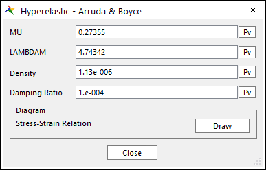
Figure 9.60 Hyperelastic - Arruda & Boyce dialog box

• MU ( \(\mu\) ): The initial shear modulus.

• LAMBDAM ( \({{\lambda }_{M}}\) ): The maximum (locking) stretch of the material. (\({{\lambda }_{M}}=\sqrt{N}\))

• Strain Energy Density Function:

  \(\begin{aligned} U=\mu \left[ \cfrac{1}{2} \right. & \left. \left( {{{\bar{I}}}_{1}}-3 \right)+\cfrac{1}{20N}\left( {{{\bar{I}}}_{1}}^{2}-9 \right)+\cfrac{11}{1050{{N}^{2}}}\left( {{{\bar{I}}}_{1}}^{3}-27 \right) \right. \\ & \left. + \cfrac{19}{7000{{N}^{3}}}\left( {{{\bar{I}}}_{1}}^{4}-81 \right)+\cfrac{519}{673750{{N}^{4}}}\left( {{{\bar{I}}}_{1}}^{5}-243 \right) \right] \\ \end{aligned}\)

• Stress-Strain Relation: Under the condition that element volume does not change and uni-axial stress, strain-stress formulation is induced from strain-energy formula. Here, strain(\({{\varepsilon }_{x}}\)) and stress(\({{\sigma }_{x}}\)) indicate nominal strain and nominal stress.

  \({{\sigma }_{x}}=2{W}_{\bar{I}_{1}}\left( \lambda -{{\lambda }^{-2}} \right)\)

  \({W}_{\bar{I}_{1}}=\mu \left( \cfrac{1}{2}+\cfrac{1}{10N}{{{\bar{I}}}_{1}}+\cfrac{11}{350{{N}^{2}}}{{{\bar{I}}}_{1}}^{2}+\cfrac{19}{1750{{N}^{3}}}{{{\bar{I}}}_{1}}^{3}+\cfrac{519}{134750{{N}^{4}}}{{{\bar{I}}}_{1}}^{4} \right)\)

  \({{{\bar{I}}}_{1}}={{\lambda }^{2}}+2{{\lambda }^{-1}}\)

  \(\lambda ={{\varepsilon }_{x}}+1\)

  

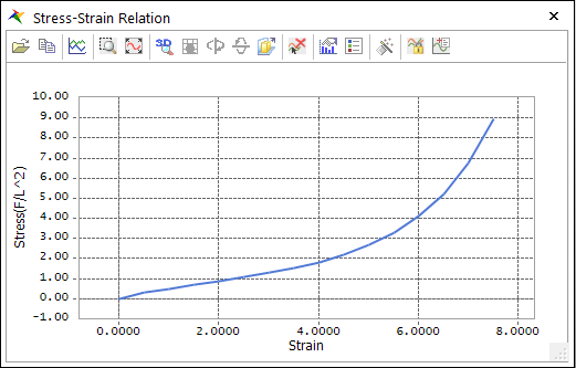
  Figure 9.61 Hyperelastic – Arruda & Boyce stress-strain plot dialog box

• Rubber Material Data:

  \(\begin{aligned} & \mu =0.27355 \\ & {{\lambda }_{M}}=4.74342 \\ \end{aligned}\)

• It is reasonable at all strain ranges in default coefficient.

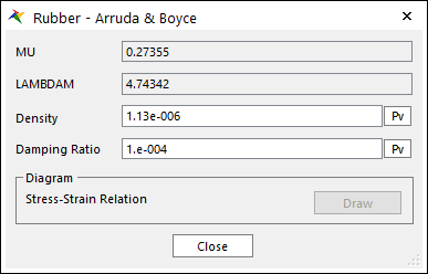
Figure 9.62 Rubber – Arruda & Boyce dialog box

9.7.4.2.2. Neo-Hooke

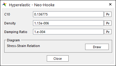
Figure 9.63 Hyperelastic - Neo-Hooke dialog box

• \(C_{10}\): The Neo-Hookean material parameter.

  The initial shear modulus \(\mu\) is given by the equation:

  \(\mu =2{{C}_{10}}\)

• Strain Energy Density Function:

  \(U={{C}_{10}}\left( {{{\bar{I}}}_{1}}-3 \right)\)

• Stress-Strain Relation: Under the condition that element volume does not change and uni-axial stress, strain-stress formulation is induced from strain-energy formula. Here, strain(\({{\varepsilon }_{x}}\)) and stress(\({{\sigma }_{x}}\)) indicate nominal strain and nominal stress.

  \(\begin{aligned} & {{\sigma }_{x}}=2{{C}_{10}}\left( \lambda -\frac{1}{{{\lambda }^{2}}} \right) \\ & \lambda ={{\varepsilon }_{x}}+1 \\ \end{aligned}\)

  

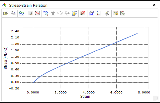
  Figure 9.64 Hyperelastic - Neo-Hooke stress-strain plot dialog box

• Rubber Material Data:

  \({{C}_{10}}=0.136775\)

• It is reasonable at low strains and the stresses are underestimated compared to Mooney-Rivlin in default coefficient.

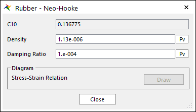
Figure 9.65 Rubber - Neo-Hooke dialog box

9.7.4.2.3. Ogden

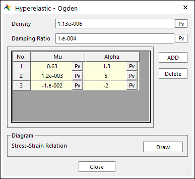
Figure 9.66 Hyperelastic - Ogden dialog box

• Mu (\(\mu\)) and Alpha (\(\alpha\)): Ogden parameters.

  At least 1 pair must be defined.

  At most 6 pairs of Mu and Alpha can be defined.

  The initial shear modulus \(\mu\) is given by the equation.

  \(2\mu =\sum\limits_{i=1}^{N}{{{\mu }_{i}}{{\alpha }_{i}}}\)

  where \(N\) is the number of user-defined (\(\mu\), \(\alpha\)) pairs defined.

• Strain Energy Density Function:

  \(U=\sum\limits_{i=1}^{N}{\cfrac{{{\mu }_{i}}}{{{\alpha }_{i}}}\left( \bar{\lambda }_{1}^{{{\alpha }_{i}}}+\bar{\lambda }_{2}^{{{\alpha }_{i}}}+\bar{\lambda }_{3}^{{{\alpha }_{i}}}-3 \right)}=\sum\limits_{i=1}^{N}{\cfrac{{{\mu }_{i}}}{{{\alpha }_{i}}}\left( \bar{\xi }_{1}^{{{\alpha }_{i}}/2}+\bar{\xi }_{2}^{{{\alpha }_{i}}/2}+\bar{\xi }_{3}^{{\alpha }_{i}/2}-3 \right)}\)

• Stress-Strain Relation: Under the condition that element volume does not change and uni-axial stress, strain-stress formulation is induced from strain-energy formula. Here, strain(\({{\varepsilon }_{x}}\)) and stress(\({{\sigma }_{x}}\)) indicate nominal strain and nominal stress.

  \(\begin{aligned} & {{\sigma }_{x}}=\left[ \sum\limits_{p=1}^{N}{{{\mu }_{p}}\left( {{\lambda }^{{{\alpha }_{p}}}}-{{\lambda }^{-\frac{1}{2}{{\alpha }_{p}}}} \right)} \right]{{\lambda }^{-1}} \\ & \lambda ={{\varepsilon }_{x}}+1 \\ \end{aligned}\)

  

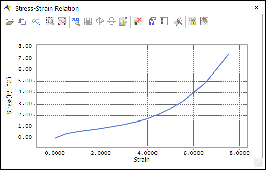
  Figure 9.67 Hyperelastic - Ogden stress-strain plot dialog box

• Rubber Material Data:

  \(\begin{aligned} & {{\mu }_{1}}=0.63,{{\mu }_{2}}=0.0012,{{\mu }_{3}}=-0.01 \\ & {{\alpha }_{1}}=1.3,{{\alpha }_{2}}=5.0,{{\alpha }_{3}}=-2.0 \\ \end{aligned}\)

• It is reliable at all strain ranges and more accurate than Arruda-Boyce in default coefficient.

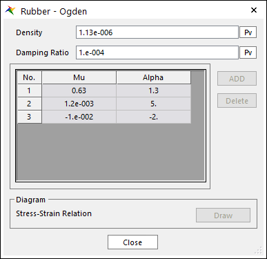
Figure 9.68 Rubber - Ogden dialog box

9.7.4.2.4. Mooney Rivlin

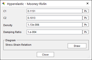
Figure 9.69 Hyperelastic – Mooney Rivlin dialog box

• C1 and C2: The Mooney-Rivlin parameters.

  The initial shear modulus \(\mu\) is given by the equation.

  \(\mu =2\left( {{C}_{1}}+{{C}_{2}} \right)\)

• Strain Energy Density Function:

  \(U={{C}_{1}}\left( {{{\bar{I}}}_{1}}-3 \right)+{{C}_{2}}\left( {{{\bar{I}}}_{2}}-3 \right)\)

• Stress-Strain Relation: Under the condition that element volume does not change and uni-axial stress, strain-stress formulation is induced from strain-energy formula. Here, strain(\({{\varepsilon }_{x}}\)) and stress(\({{\sigma }_{x}}\)) indicate nominal strain and nominal stress.

  \(\begin{aligned} & {{\sigma }_{x}}=\left( 2{{c}_{1}}+\frac{2{{c}_{2}}}{\lambda } \right)\left( \lambda -{{\lambda }^{-2}} \right) \\ & \lambda ={{\varepsilon }_{x}}+1 \\ \end{aligned}\)

  

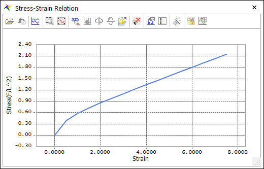
  Figure 9.70 Hyperelastic - Mooney Rivlin stress-strain plot dialog box

• Rubber Material Data:

  \(\begin{aligned} & {{C}_{1}}=0.1151 \\ & {{C}_{2}}=0.1013 \\ \end{aligned}\)

• It is reasonable at low strains and the stresses are overestimated compared to Neo-Hooke in default coefficient.

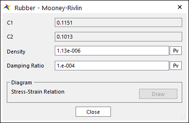
Figure 9.71 Rubber – Mooney-Rivlin dialog box