14.2.2.1. Axial Mode

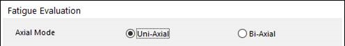
Figure 14.9 Fatigue Evaluation dialog box

The user can select the Uni-Axial mode or the Bi-Axial mode.

• Uni-Axial

  • In order to make durability assessments more efficient, fatigue properties obtained using standard specimens in a controlled laboratory environment are commonly used to predict fatigue damage and life using the strain histories measured by strain gauges mounted on critical areas of the structures.

  • At that time, the loading direction of a specimen is just one direction with the tensile and compressive motion. So, the general or traditional fatigue analysis regards the axial direction as one.

• Bi-Axial

  • Many real engineering design situations require multi-axial fatigue equations, for example rotating shafts, connecting links, automotive and aircraft components and so on. The multi-axial effects complicate the analysis required for the prediction of fatigue behavior.

  • Bi-Axial method is commonly used for multi-axial fatigue evaluations. This method can define lateral loading, what we call the biaxial ratio, in stress or strain time history. At that time, several life criteria such as mostly stress life assume that the loading is proportional, so that it can count the stress or strain cycles in one direction and decide the corresponding ones in other direction. This method is called the bi-axiality ratio method or Von Mises Effective Amplitude Approach.

  • For biaxial fatigue evaluation, it is assumed that the loading is proportional and that there is a constant ratio between the stresses on two principal axes. However, in a general event, the loading may not be proportional, and the stress ratio actually changes from time to time. At this point, the linear square method is used to determine the stress/strain biaxial ratio as following equations:

    \(\gamma =\frac{{{\sum\nolimits_{i}^{n}{\left( {{\sigma }_{x}}\cdot {{\sigma }_{y}} \right)}}_{i}}}{{{\sum\nolimits_{i}^{n}{\left( {{\sigma }_{x}}\cdot {{\sigma }_{x}} \right)}}_{i}}}\) or \(\gamma =\frac{{{\sum\nolimits_{i}^{n}{\left( {{\varepsilon }_{x}}\cdot {{\varepsilon }_{y}} \right)}}_{i}}}{{{\sum\nolimits_{i}^{n}{\left( {{\varepsilon }_{x}}\cdot {{\varepsilon }_{x}} \right)}}_{i}}}\)

    Where, i represents each time step and n means the total number of time step. \({{\sigma }_{x}}\) and \({{\sigma }_{y}}\) mean the stress in the primary and secondary loading direction.

  • This approach is used for stress life (Manson-Coffin, ASME, BWI) and strain life(Manson-Coffin, Morrow, SWT).

  • Another Bi-Axial method is the critical plane method or Brown-Miller Approach which is used for the maximum shear strain components. First of all, this method decides the critical (maximum shear strain) plane using the three principal axes on the element face. It then calculates the maximum shear cycle in the constant shear direction on the critical plane. A constant ratio(c) is used to determine the corresponding normal strain cycle (normal to the maximum shear direction) for each identified maximum shear strain cycle.

  • The bi-axiality ratio method calculates fatigue results quickly. But it becomes too conservative when the loading between the two axes is not proportional. However, the critical plane method takes a lot of time in searching the critical plane, but it is more accurate than the other method.

Note

The Bi-Axial mode is recommended because the realistic excitation is a multi-axial type.