14.2.2.5. Time History
In order to evaluate the fatigue results, it is necessary to get the stress/strain results based on time. However, if all time history is selected in case of a lot of animation frames after simulation, it takes long time to calculate the fatigue results. Therefore, RecurDyn/Durability has supported the user-defined time history as shown in the Figure 14.26. In addition, if you want to separate the time history as several time sets, it is needed to support to define the mulit-time sets. So,

Figure 14.24 The Time History section in the Fatigue Evaluation dialog
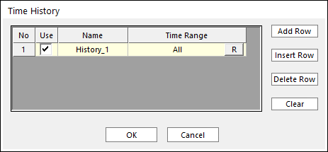
Figure 14.25 The Time History dialog
If SEL is clicked in the Time History section in the Fatigue Evaluation dialog as shown in the Figure 14.24, the Time History dialog appears as shown in the Figure 14.25. In this dialog, if the time history is added or subtracted or modified, the several buttons such as Add Row, Insert Row, Delete Row and Clear help you work. In addition, it is possible to define new name of time history in the Name section whenever the new time history is added. And in order to be available the defined time history, you the Use checkbox should be selected. And then, the defined multi-time history sets are shown as the defined name of each time history as shown in the Figure 14.26.
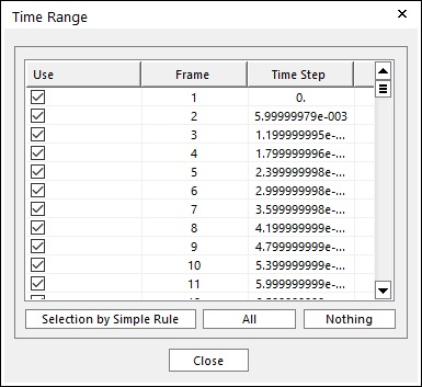
Figure 14.26 The way to define time set in Time Range
If the user clicks R for Time History, the Time Range dialog box is opened. Using this dialog, the user can compose the Time history cycle for the evaluation. In order to compose the cycle, the user can select the Use checkbox individually or the user can use Selection by Simple Rule, All, or Nothing.
Selection by Simple Rule: Allows the user to open the Selection dialog box to support a simple rule selecting many sheet bodies at the same time.
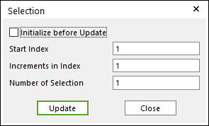
Figure 14.27 Selection dialog box
\(N_{selection} = N_{start} + \Delta * (i-1) , i = 1,...,n\)
Initialize before Update: If this button is checked and click the Update, only the check boxes of links selected by user-defined rule are activated. Or not, the check boxes of pre-selected links and links selected by user-defined rule are activated.
Start Index: Shows the starting index in the simple rule.
Increment in Index: Shows the increment of index in the simple rule.
Number of Selection: Shows the number of selected links in the simple rule.
The reason why it is necessary to use Time History is it takes long time to calculate fatigue results by using the original time history that is obtained after simulation. In other words, as shown in the figure below, the original time history can be changed to the selected time history by using Time History. And then, it is possible for RecurDyn/Durability solver to do Rainflow Counting with the selected time history that is defined by user.
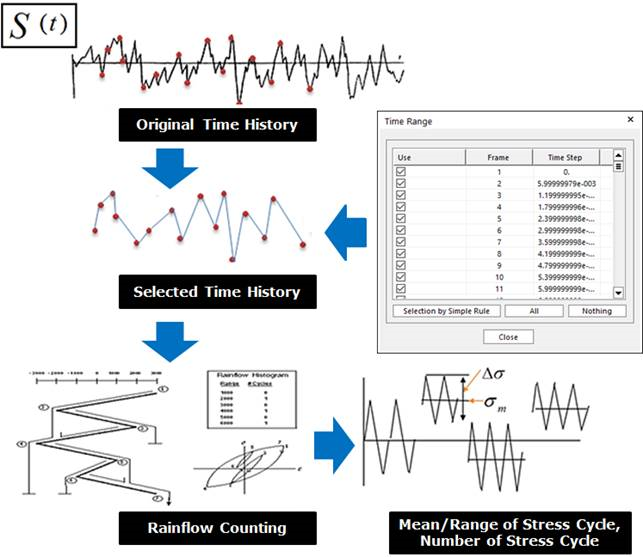
Figure 14.28 The procedure for Rainflow Counting
Rainflow Counting is the most popular counting method in fatigue life estimation because it follows the stress-strain hysteresis loop. This counting method was named rainflow by its inventors, M. Matsuishi and T. Endo, because graphically it looks similar to rain flowing down a pagoda roof. This method is the most well accepted and commonly used counting method among the different methods to identity and count fatigue cycles. Using the Rainflow counting, a time history is re-sequenced into various numbers of fatigue loading cycles of stress (or strain) amplitudes with mean stresses. Once the loading cycles are identified and the number of cycles counted, the fatigue damage of each cycle can be calculated and then linearly combined into a cumulative damage for the whole loading history.
RecurDyn/Durability supports to show the results of Rainflow Counting in an Excel spreadsheet. In the Excel spreadsheet, it is possible for users to see easily the stress/strain range, the mean stress/strain and the number of cycles from the defined time history a 3D chart as shown below Figure 14.29. In addition, the raw data to draw the chart can be shown in the Excel.
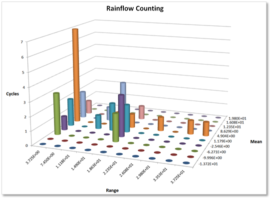
Figure 14.29 The Rainflow Counting results in a 3D chart