21.3.5. Guides for Multi-Objective Optimization
Multi-objective optimization strategy gives non-unique solution. Let’s consider the typical optimization formulation as
\(\underset{\mathbf{x}}{\mathop{\min }}\,P\left( {{f}_{i}}\left( \mathbf{x} \right) \right),\text{ }i=1,2,...,m\)
Where, the design variable vector \(\mathbf{x}\) belong to the feasible set \(\Omega \subset {{R}^{n}}\), defined by equality and inequality constraints as \(\Omega =\left\{ \mathbf{x}\in {{R}^{n}}:\mathbf{h}\left( \mathbf{x} \right)=\mathbf{0},\mathbf{g}\left( \mathbf{x} \right)\le \mathbf{0} \right\}\). Also, \({{f}_{i}}\left( \mathbf{x} \right)\) is the ith objective and the functional \(P\) is called as a preference function.
Unlike a single objective, multi-objective optimization has no unique solution that would give an optimum for all objectives simultaneously. We call it as a Pareto optimal. A solution \({{\mathbf{x}}^{*}}\) is Pareto optimal if there exists no feasible point \(\mathbf{x}\) which would decrease some objectives without causing a simultaneously increase in at least one objective. Figure 21.78 shows the Pareto optimum.
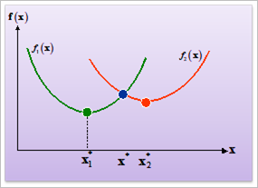
Figure 21.78 Local Pareto optimum in two objective case
Two points \(\mathbf{x}_{1}^{*}\) and \(\mathbf{x}_{2}^{*}\) are local optima for objectives \({{f}_{1}}\left( \mathbf{x} \right)\) and \({{f}_{2}}\left( \mathbf{x} \right)\), respectively. In multi-objective optimization, they are called as an ideal optimum and the point \({{\mathbf{x}}^{*}}\) is a local Pareto optimum.