9.10.2. Stress-Strain Relationships

This section discusses the Stress-Strain relationships for linear materials and nonlinear materials as they are applied in RecurDyn.

9.10.2.1. Strain measure

The strain measure of both linear and nonlinear materials is the same by strain definition.

The Green strain tensor:

• Is the most widely used in nonlinear finite element method.

• Is expressed in terms of displacement gradients as follows.

  \({{\varepsilon }_{ij}}=\cfrac{1}{2}\left( \cfrac{\partial {{u}_{i}}}{\partial {{x}_{j}}}+\cfrac{\partial {{u}_{j}}}{\partial {{x}_{i}}}+\cfrac{\partial {{u}_{k}}}{\partial {{x}_{i}}}\cfrac{\partial {{u}_{k}}}{\partial {{x}_{j}}} \right)\)

  The strain vector is written as follows:

  \(\left\{ \varepsilon \right\}={{\left[ {{\varepsilon }_{x}}{{\varepsilon }_{y}}{{\varepsilon }_{z}}{{\gamma }_{xy}}{{\gamma }_{yz}}{{\gamma }_{zx}} \right]}^{T}}\)

  For linear elasticity, the strain components are the first order derivatives of displacement components as shown below:

  \(\left\{ \varepsilon \right\}=\left\{ \begin{aligned} & {{\varepsilon }_{x}} \\ & {{\varepsilon }_{y}} \\ & {{\varepsilon }_{z}} \\ & {{\gamma }_{xy}} \\ & {{\gamma }_{yz}} \\ & {{\gamma }_{zx}} \\ \end{aligned} \right\}=\left[ \begin{matrix} \cfrac{\partial }{\partial x} & 0 & 0 \\ 0 & \cfrac{\partial }{\partial y} & 0 \\ 0 & 0 & \cfrac{\partial }{\partial z} \\ \cfrac{\partial }{\partial y} & \cfrac{\partial }{\partial x} & 0 \\ 0 & \cfrac{\partial }{\partial z} & \cfrac{\partial }{\partial y} \\ \cfrac{\partial }{\partial z} & 0 & \cfrac{\partial }{\partial x} \\ \end{matrix} \right]\left\{ \begin{aligned} & u \\ & v \\ & w \\ \end{aligned} \right\}\)

9.10.2.2. Stress measure

The stress vector is related to the strain vector by a constitutive relationship that indicates the elastic properties of FFlex body.

\(\left\{ \sigma \right\}=\left[ \mathbf{D} \right]\left\{ \varepsilon \right\}\)

The stress components are expressed in the vector form.

\(\left\{ \sigma \right\}={{\left[ {{\sigma }_{x}}{{\sigma }_{y}}{{\sigma }_{z}}{{\tau }_{xy}}{{\tau }_{yz}}{{\tau }_{zx}} \right]}^{T}}\)

9.10.2.2.1. Linear materials

The stress vectors are shown in Figure 9.168 below. The sign convention for direct stresses and strains is that tension is positive, and compression is negative. For shears, positive is when the two applicable positive axes rotate toward each other.

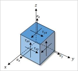
Figure 9.168 Three-dimensional Stress Components

The elasticity matrix \(\left[ \mathbf{D} \right]\) is symmetric. For isotropic materials, all of the terms of \(\left[ \mathbf{D} \right]\) depend on only two elastic constants: the elastic modulus (\(E\)) and Poisson’s ratio (\(\nu\)). For the isotropic case:

\(\left\{ \begin{matrix} {{\sigma }_{x}} \\ {{\sigma }_{y}} \\ {{\sigma }_{xy}} \\ \end{matrix} \right\}=\left[ \mathbf{D} \right]\left\{ \mathbf{\varepsilon } \right\}=\left[ \begin{matrix} \cfrac{E}{\left( 1-{{\nu}^{2}} \right)} & \cfrac{E\nu}{\left( 1-{{\nu}^{2}} \right)} & 0 \\ \cfrac{E\nu}{\left( 1-{{\nu}^{2}} \right)} & \cfrac{E}{\left( 1-{{\nu}^{2}} \right)} & 0 \\ 0 & 0 & \cfrac{E}{2\left( 1+\nu \right)} \\ \end{matrix} \right]\left\{ \begin{matrix} {{\varepsilon }_{x}} \\ {{\varepsilon }_{y}} \\ {{\gamma }_{xy}} \\ \end{matrix} \right\}\) (Shell element)

\(\left\{ {{\mathbf{\sigma }}_{{{p}_{2}}}} \right\}=\left[ \mathbf{D} \right]\left\{ \mathbf{\varepsilon } \right\}=\cfrac{E}{\left( 1+\nu \right)\left( 1-2\nu \right)}\left[ \begin{matrix} 1-\nu & \nu & \nu & 0 & 0 & 0 \\ {} & 1-\nu & \nu & 0 & 0 & 0 \\ {} & {} & 1-\nu & 0 & 0 & 0 \\ {} & {} & {} & \frac{1-2\nu }{2} & 0 & 0 \\ {} & {} & {} & {} & \frac{1-2\nu }{2} & 0 \\ {} & {} & {} & {} & {} & \frac{1-2\nu }{2} \\ \end{matrix} \right]\left\{ \begin{matrix} {{\varepsilon }_{x}} \\ {{\varepsilon }_{y}} \\ {{\varepsilon }_{z}} \\ {{\gamma }_{xy}} \\ {{\gamma }_{yz}} \\ {{\gamma }_{zx}} \\ \end{matrix} \right\}\) (Solid element)

9.10.2.2.2. Nonlinear material

Hyperelastic

When the constitutive relationship is expressed in terms of the strain energy density function, WD, the stress-stretch behavior is found by differentiation with respect to the stretch. For the case of purely incompressibility, the principal Cauchy stresses, \({{\sigma }_{i}}\) are found by differentiating with respect to the principle stretches, \({{\lambda }_{i}}\)

\({{\sigma }_{i}}={{\lambda }_{i}}\left[ \cfrac{\partial {{W}_{D}}}{\partial {{I}_{1}}}\cfrac{\partial {{I}_{1}}}{\partial {{\lambda }_{i}}}+\cfrac{\partial {{W}_{D}}}{\partial {{I}_{2}}}\cfrac{\partial {{I}_{2}}}{\partial {{\lambda }_{i}}} \right]+\hat{p},(i=1,2,3)\)

Where,

\({{W}_{D}}=U-\hat{p}\,(J-1)\) : Energy density function

\(U\) : Strain energy of each material type

\(J=\det (\mathbf{F})\) : Volume change

\(\mathbf{F}\) : Displacement gradient

\(\hat{p}\) : Lagrange multiplier

\({{\lambda }_{i}}\) : Principle stretches

\(\mathbf{B}=\mathbf{F}{{\mathbf{F}}^{\text{T}}}\) : Left Cauchy-Green displacement tensor

\({{I}_{1}},\,{{I}_{2}}\) : Invariant of \(\mathbf{B}\)

\({{I}_{1}}=\lambda _{1}^{2}+\lambda _{2}^{2}+\lambda _{3}^{2}\):

\({{I}_{2}}=\lambda _{1}^{2}\lambda _{2}^{2}+\lambda _{2}^{2}\lambda _{3}^{2}+\lambda _{3}^{2}\lambda _{1}^{2}\):

Cauchy stress tensor is expressed with principal Cauchy stress tensor and orientation matrix.

\(\boldsymbol{\sigma} ={{\mathbf{A}}^{T}}\left[ \begin{matrix} {{\sigma }_{1}} & 0 & 0 \\ 0 & {{\sigma }_{2}} & 0 \\ 0 & 0 & {{\sigma }_{3}} \\ \end{matrix} \right]\mathbf{A}=\left[ \begin{matrix} {{\sigma }_{xx}} & {{\tau }_{xy}} & {{\tau }_{xz}} \\ {{\tau }_{yx}} & {{\sigma }_{yy}} & {{\tau }_{yz}} \\ {{\tau }_{zx}} & {{\tau }_{zy}} & {{\sigma }_{zz}} \\ \end{matrix} \right]\)

The stress components can also be expressed in vector for

\(\left\{ \boldsymbol{\sigma } \right\}={{[{{\sigma }_{x}} \, {{\sigma }_{y}} \, {{\tau }_{xy}} \, {{\tau }_{yz}} \, {{\tau }_{zx}}]}^{T}}\)

9.10.2.3. Principal Strain, Principal Stress

• The principal strains and stresses are calculated from the strain tensor and the stress tensor, respectively.

• The intensity is the largest absolute values of principal values.

• The von Mises stress is computed from the principal values.

  Table 9.10 :header-rows: 1 :widths: 20 40 40

  	Strain	Stress
  Tensor	\(\varepsilon_{x}\,\), \(\varepsilon_{y}\,\), \(\varepsilon_{z}\,\), \(\varepsilon_{xy}\,\), \(\varepsilon_{yz}\,\), \(\varepsilon_{zx}\)	\(\sigma_{x}\,\), \(\sigma_{y}\,\), \(\sigma_{z}\,\), \(\sigma_{xy}\,\), \(\sigma_{yz}\,\), \(\sigma_{zx}\)
  Principal	\(\varepsilon_{1}\,\), \(\varepsilon_{2}\,\), \(\varepsilon_{3}\)	\(\sigma_{1}\,\), \(\sigma_{2}\,\), \(\sigma_{3}\)
  Intensity	\(\varepsilon_{I}=\text{max}(|\varepsilon_1-\varepsilon_2|,|\varepsilon_2-\varepsilon_3|,|\varepsilon_3-\varepsilon_1|)\)	\(\sigma_{I}=\text{max}(|\sigma_1-\sigma_2|,|\sigma_2-\sigma_3|,|\sigma_3-\sigma_1|)\)
  von Mises	\(\varepsilon_{e}=\left(\frac{2}{9} [(\varepsilon_1-\varepsilon_2)^2+(\varepsilon_2-\varepsilon_3)^2+(\varepsilon_3-\varepsilon_1)^2]\right) ^{1/2}\)	\(\sigma_{e}=\left(\frac{1}{2} [(\sigma_1-\sigma_2)^2+(\sigma_2-\sigma_3)^2+(\sigma_3-\sigma_1)^2]\right) ^{1/2}\)