7.2.1.4. FFT
7.2.1.4.1. Definition of FFT Analysis
FFT(Fast Fourier Transform) is a mathematical algorithm that takes a time-domain data and maps it into its frequency-domain.
Discrete Fourier Transform
Suppose that we have N consecutive sampled values
\(h_k \equiv h(t_k), t_k \equiv k\Delta, k=0,1,2,...,N-1\)
so that the sampling interval is \(\Delta\). To make things simpler, let us also suppose that N is even. With N numbers of input, we can estimate the Fourier transform \(H(f)\) at the discrete values.
\(f_n \equiv \frac{n}{N \Delta}, n=-\frac{N}{2},...,\frac{N}{2}\)
The extreme values of n correspond exactly to the lower and upper limits of the Nyquist critical frequency range.
The Fourier transform is approximated by a discrete sum. The discrete Fourier transform is obtained as,
\(H(f_n)=\int _{-\infty}^{\infty} h(t)e^{-2\pi \dot{\omega_n}t}dt \approx \sum _{k=0}^{N-1}h_ke^{-2 \pi \dot{\omega_n}} \Delta = \Delta \sum _{k=0}^{N-1}h_ke^{-2\pi \dot{\omega_n} /N}\)
If the number of sampled values is an even power of two (for example, 256, 512, 1024, and so on), the discrete Fourier transform can be computed in \(O(Nlog_2N)\) operations with an algorithm called the fast Fourier transform, or FFT.
Magnitude
FFT/magnitude determines the magnitude (abs) of the complex value returned from the FFT algorithm.
Phase
FFT/Phase determines the phase angle of the complex value returned from the standard FFT algorithm.
Power Spectral Density (PSD)
FFT/Power Spectral Density determines the periodogram estimation of the complex value returned from the standard FFT algorithm. If we take an N point sample of the function c(t) at equal intervals and use the FFT to compute its discrete Fourier transform
\(C_k=\sum _{i=0}^{N-1}c_ie^{-2\pi \dot{\omega_n} /N} , k=0,...,N-1\)
Then the periodogram estimate for the Spectrum type is defined at N/2+1 frequencies as
\(P(0)=P(f_0)=\frac{1}{N^2} \left| C_0 \right|^2\)
\(P(f_k)=\frac{1}{N62}\left[ |C_k|^2 + |C_{N-k}|^2 \right] k=1,2,...,(\frac{N}{2}-1)\)
\(P(f_c)=P(f_{N/2})=\frac{1}{N^2}|C_{N/2}|^2\)
where, \(f_k\) is defined only for the zero and positive frequencies
\(f_k \equiv \frac{k}{N\Delta}=2f_c\frac{k}{N}, k=-\frac{N}{2},...,\frac{N}{2}\)
where, \(\Delta\) and \({{f}_{c}}\) are the sampling interval and the Nyquist frequency (=half of the sampling frequency), respectively.
PSD Type: The PSD Type is a scaling option. There are two options as Spectrum and Density.
The Spectrum type is default. And the result is normalized to the unit time. If the target signal unit is defined as [v], then the unit of the Spectrum result is defined as [\(\nu^2\)].
\(P(0)=P(f_0)=\frac{1}{N^2} \left| C_0 \right|^2\)
\(P(f_k)=\frac{1}{N62}\left[ |C_k|^2 + |C_{N-k}|^2 \right] , k=1,2,...,(\frac{N}{2}-1)\)
\(P(f_c)=P(f_{N/2})=\frac{1}{N^2}|C_{N/2}|^2\)
The Density type is a scaled result from the Spectrum result multiplied by the ratio of the number of the data and sampling frequency. If the target signal unit is defined as [v], then the unit of the Spectrum result is defined as [\(\frac{\nu^2}{Hz}\)].
\(P_{Density}(f)=P(f)\frac{N}{2f_c}=P(f)N\Delta\)
Window Method
The time-domain data is assumed a periodic sample from a continuous, infinite series of data for FFT. Window methods are used to reduce discontinuities from mismatching start and end and ensure periodicity of the FFT conditions.
The functions of window methods are defined below. In the equation, \(W_j\) is the function of the window method and N is the number of sampled values.
Square Window
\({{W}_{j}}=1\)
Bartlett Widow
\({{W}_{j}}=1-\left| \frac{j-\frac{N-1}{2}}{\frac{N}{2}} \right|\)
Welch Window
\({{W}_{j}}=1-{{\left( \frac{j-\frac{N-1}{2}}{\frac{N+1}{2}} \right)}^{2}}\)
Hanning Window
\({{W}_{j}}=\frac{1}{2}\left( 1-\cos \left( \frac{2\pi j}{N-1} \right) \right)\)
Hamming Window
\({{W}_{j}}=0.54-0.46\times \cos \left( \frac{2\pi j}{N-1} \right)\)
Blackman
\({{W}_{j}}=0.42-0.5\times \cos \left( \frac{2\pi j}{N-1} \right)+0.08\times \cos \left( \frac{4\pi j}{N-1} \right)\)
7.2.1.4.2. Property
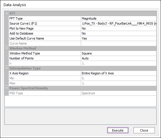
Figure 7.55 Data Analysis dialog box [FFT]
FFT
FFT Type: Selects a type of FFT.
Magnitude
Phase
Power Spectral Density
Source Curve: Selects a curve.
Plot to New Page: If the user wants to draw to a new page, select Yes. If the user wants to draw to the current page, select No. (The default option is No.)
Add to Database: If the user wants to add a desired result to the database, select Yes. (The default option is No.)
Use Default Curve Name: If you want to use the default curve name like “ADD(Acc_TM-Body1(mm/s^2), Vel_TM-Body1(mm/s))”, select Yes. If not, the Chart use the Curve Name.
Curve Name: If Use Default Curve Name is No, Chart use this for a name.
Window Method
Window Method Type: Selects a type of the window method.
Square
Barlett
Welch
Hanning
Hamming
Blackman
Number of Points Type: Selects a type of the number of points.
Auto
2^n
n: Number n used in 2^n.
Interpolation Type
X Axis Region
Entire Region of X Axis
Specified Region of X Axis: Set up Min and Max.
Min: Minimum X value.
Max: Maximum Y value.