21.4.6.1. Monte Carlo Simulation
Monte Carlo Simulation is a powerful engineering tool that can be used for statistical analysis of uncertainty in engineering problems. If a system parameter is known to follow certain probability distribution, the performance of the system is studied by considering several possible values of the parameter, each following the specified probability distribution. In the context of system reliability, the Monte Carlo simulation involves constructing trial systems on a computer according to generated random numbers and determining the percentage of systems that fail. Of course, a large number of trial systems are needed if high confidence is required at small failure probability levels. The Monte Carlo approach, thus, requires considerable calculations and is useful only for complex interrelated systems or for the verification of other reliability analyses.
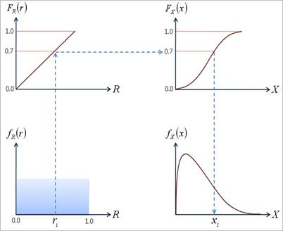
Figure 21.146 Inverse CDF method
21.4.6.1.1. Generation of Random Numbers
The generation of random numbers according to a specific distribution is the heart of Monte Carlo simulation. In general, all language compilers provide the random number generator to generate uniformly distributed random number between 0 and 1. The main task is to transform the uniform random numbers \({{r}_{i}}\) between 0 and 1 to random numbers with the appropriate characteristic. This is commonly known as the inverse transformation techniques or inverse CDF method. In this method, the CDF of the random variable is equated to the generated random number \({{r}_{i}}\), that is, \({{F}_{X}}({{x}_{i}})={{r}_{i}}\), and the equation is solved for \({{x}_{i}}\) as
\({{x}_{i}}={{F}_{X}}^{-1}({{r}_{i}})\)
21.4.6.1.2. Probabilistic Information Extraction
Let’s consider a performance function of system.
\(Z=g({{X}_{1}},{{X}_{2}},...,{{X}_{n}})\)
which describes the functional relationships among the random numbers. The failure surface or the limit state of interest can then be defined as \(z=0\). This is the boundary between the safe and failure regions in the design variable space. Suppose that \({{X}_{1}}\) and \({{X}_{2}}\) are the two basic random variables, the failure surface and the safe and failure regions are shown in Figure 21.147.
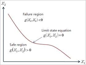
Figure 21.147 Limit state concept
The Monte Carlo simulation generates the random samples of the variables according to their PDFs and PMFs, which is described in the previous section. Then, the random response \(Z\) can be evaluated from the performance function \(g({{X}_{1}},{{X}_{2}},...,{{X}_{n}})\). Suppose that failure region is defined as \(g({{X}_{1}},{{X}_{2}},...,{{X}_{n}})<0\) shown in the Figure 21.146. Let \({{N}_{f}}\) be the number of sample points when \(g({{X}_{1}},{{X}_{2}},...,{{X}_{n}})<0\) and \(N\) be the total number of sample points. Therefore, an estimate of the probability of failure can be expressed as
\({{P}_{f}}=\frac{{{N}_{f}}}{N}\)
21.4.6.1.3. Accuracy and Efficiency of Estimation
The accuracy of the estimate of \({{P}_{f}}\) may depend on the number of sample points(\(N\)). A small number of sample points give the estimate of \({{P}_{f}}\) subject to considerable error. The estimate of probability failure would approach the true value as \(N\) approaches infinity. Thus, the accuracy of the estimation has been studied in several ways.
Variance of Estimation
One way would be to evaluate the variance or COV of the estimated probability of failure. The COV can be estimated by assuming each simulation to constitute a Bernoulli trial, and the number of failure(\({{N}_{f}}\)) in \(N\) trials can be considered to follow a binomial distribution. Then, the COV of the estimate \({{P}_{f}}\) can be defined as
\(COV({{P}_{f}})\approx \frac{\sqrt{\frac{(1-{{P}_{f}}){{P}_{f}}}{N}}}{{{P}_{f}}}\)
When you compare the results of Monte Carlo Simulation, a smaller value of \(COV({{P}_{f}})\) is more accurate result of them. The above equation represents that COV approaches zero as \(N\) approaches infinity.
Confidence Interval of Estimation
Another way to study the error associated with the number of simulations is by approximating the binomial distribution with a normal distribution and estimating the \((1-a)\%\) confidence interval of the estimated probability of failure. It can be defined as
\(\Pr ob\left[ -2\sqrt{\frac{(1-P_{f}^{*})P_{f}^{*}}{N}<\frac{{{N}_{f}}}{N}}-{{P}_{f}}^{*}<2\sqrt{\frac{(1-P_{f}^{*})P_{f}^{*}}{N}} \right]=1-a\)
where \(P_{f}^{*}\) is the exact probability of failure. The percentage error of the probability of failure can be defined as
\(\varepsilon =\frac{\frac{{{N}_{f}}}{N}-P_{f}^{*}}{P_{f}^{*}}\times 100\)
Combining those two equations, the percentage error can be simplified as
\(\varepsilon =100\times {{\Phi }^{-1}}(1-\frac{a}{2})\sqrt{\frac{(1-P_{f}^{*})}{N\times P_{f}^{*}}}(\%)\)
For example, for 10% error with 95% confidence, the required number of samples is
\(N=396\left( \frac{1-P_{f}^{*}}{P_{f}^{*}} \right)\)
If \(P_{f}^{*}\) is 0.01, then the required \(N\) is 39,204 for 10% error with 95% confidence. Table 21.12 lists the required samples for 10% error with 95% confidence interval.
Prob |
0.01 |
0.02 |
0.03 |
0.04 |
0.05 |
0.1 |
0.2 |
0.3 |
0.4 |
0.5 |
N |
39204 |
19404 |
12804 |
9504 |
7524 |
3564 |
1584 |
924 |
594 |
396 |
21.4.6.1.4. Example for Normal Distributions
The performance function of a mechanical system is given by
\(Z=g({{x}_{1}},{{x}_{2}})={{x}_{1}}^{3}+{{x}_{2}}^{3}-18\)
Where \({{x}_{1}}\) and \({{x}_{2}}\) are the random variables with normal distributions. Their mean values and standard deviation values are (10,10) and (5,5), respectively. If the performance function, \(Z>0\), then the system is always safe. Find the probability of failure for the mechanical system.
Sol: Figure 21.148 , Figure 21.149, Figure 21.150, and Figure 21.151 show the results of Monte Carlo Simulation. Monte-Carlo simulation of AutoReliability provides two sampling methods such as the latin hypercube sampling and the random sampling. In this study, the Latin Hypercube sampling is employed. As the number of sample points is increased, the probability is more accurate.
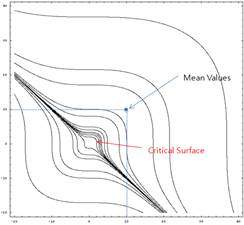
Figure 21.148 Critical surface [Analysis results of Monte Carlo Simulations]
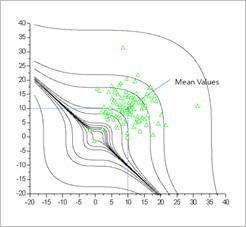
Figure 21.149 Monte Carlo Simulation (N=100, Prob=0.01, COV=0.99) [Analysis results of Monte Carlo Simulations]
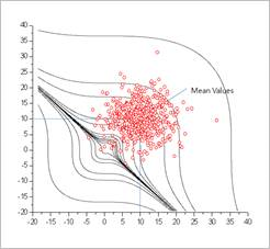
Figure 21.150 Monte Carlo Simulation (N=500, Prob=0.01, COV=0.44) [Analysis results of Monte Carlo Simulations]
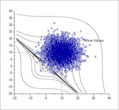
Figure 21.151 Monte Carlo Simulation (N=5000, Prob=0.0068, COV=0.17) [Analysis results of Monte Carlo Simulations]
The sample points of Figure 21.151 showed the characteristic of Inverse CDF method clearly. Even though the random sample points are selected between 0 and 1, the inverse CDF transformation makes the real sample points distributed in their statistical distributions.
Suppose that the distributions of sample points are cut at \({{x}_{1}}=10\) and \({{x}_{2}}=10\). As you can see, the shapes of distribution ware normal distributions.
21.4.6.1.5. Example for Weibull and Extreme Value Distributions
Consider the following example in which \(Z\) is linear in the two basic variables \({{x}_{1}}\) and \({{x}_{2}}\).
\(Z=g({{x}_{1}},{{x}_{2}})={{x}_{1}}-{{x}_{2}}\)
In which here \({{x}_{1}}\) is Weibull distribution and \({{x}_{2}}\) is the maximum distribution of extreme value. Their mean and standard deviation values are (20,10) and (3,3), respectively.
Sol: Figure 21.152 shows the result of Monte Carlo simulation with 1000 latin hypercube samples. The probability of failure is estimated as 0.021. As you can see, the distribution of sample points is quite different from those shown in the Figure 21.151.
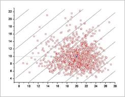
Figure 21.152 Monte Carlo simulation for Weibull and EVD-I max distributions
Next, let’s compare the sample point distributions by changing the statistical distribution. Suppose that \({{x}_{2}}\) is normal distribution for the above problem. For fair comparisons, the same random points between 0 and 1 are used. Figure 21.153 shows the real sample points. If we cut the distribution at \({{x}_{1}}=20\), the sample points are nearly symmetric distributions along \({{x}_{2}}\) axis. The vertical axis is \({{x}_{2}}\). As the statistical distribution is changed, the probability of failure is changed as 0.011.
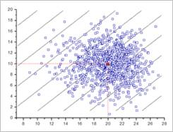
Figure 21.153 Monte Carlo simulation for Weibull and Normal distributions
Reference
Achintya Haldar and Sankaran Mahadevan, Probability, Reliability, and Statistical Methods in Engineering Design, John Wiley & Sons, Inc., New York, 2000.
Singiresu S. Rao, Reliability-Based Design, McGraw-Hill, Inc., New York, 1992.
Harbitz, A., “An Efficient Sampling Method for Probability of Failure Calculation, ”Structural Safety, Vol. 3, pp. 109-115, 1986.
Ang, A.H.-S., and Tang, W.H., Probability Concepts in Engineering Planning and Design, Volume II: Decision, Risk, and Reliability, John Wiley & Sons, Inc., New York, 1984.
Wang, L. and Grandhi, R.V., “Efficient Safety Index Calculation for Structural Reliability Analysis”, Computer & Structures Vol. 52, No. 1, pp. 103-111, 1994.
Wu Y.-T., and Wirsching, P.-H., “New Algorithm for Structural Reliability Estimation”, ASCE Journal of Engineering Mechanics, Vol. 113, No.9, pp. 1319-1336,