21.4.3.3. Response Surface Method
Response surface Method is an integration of statistical and mathematical techniques useful for developing, improving, and optimizing process. The most extensive applications of RSM are in the industrial world, particularly in situations where several variables potentially influence some performance measure or quality characteristics of the product or process. In general, a product or system response \(y\) depends on the controllable input variables \({{x}_{1}},\text{ }{{x}_{2}},\text{ }...,\text{ }{{x}_{k}}\). The relationship is
\(y=f\left( {{x}_{1}},\text{ }{{x}_{2}},\text{ }...\text{, }{{x}_{k}} \right)+\varepsilon\)
where, the form of true response function \(f\) is unknown and perhaps very complicated, and \(\varepsilon\) is a term that represents other sources of variability not included in \(f\). In general, the statistical error \(\varepsilon\) is a normal distribution \(N\left( 0,{{\sigma }^{2}} \right)\). Suppose that the linear model \(y\) may be represented by
\(y={{\beta }_{0}}+\sum\limits_{i=1}^{k}{{{\beta }_{i}}{{x}_{i}}}+\varepsilon\)
where, \({{\beta }_{i}}\) are the unknown coefficients. If there is more than one data point under consideration, the linear model is extended to the matrix form
\(\mathbf{Y}=\mathbf{X\beta }+\mathbf{\varepsilon }\)
where \(\mathbf{Y}\) is a vector of \(N\) observations, \(\mathbf{X}\) is a matrix of known constant, \(\mathbf{\beta }\) is a vector of \(p=k+1\) parameters, and \(\mathbf{\varepsilon }\) is the vector of random errors. In order to obtain the unknown coefficients, we solve the sum of squares of residuals as \({{S}_{e}}={{\mathbf{\varepsilon }}^{T}}\mathbf{\varepsilon }={{\left( \mathbf{Y}-\mathbf{X\beta } \right)}^{T}}\left( \mathbf{Y}-\mathbf{X\beta } \right)\). To minimize \({{S}_{e}}\), we solve a set of \(p\) equations. Hence the normal equation \(\left[ {{\mathbf{X}}^{T}}\mathbf{X} \right]\mathbf{\beta }=\left\{ {{\mathbf{X}}^{T}}\mathbf{Y} \right\}\) is obtained. The matrix \({{\mathbf{X}}^{T}}\mathbf{X}\) is a symmetric matrix with \(p\) rows and \(p\) columns. Its rank is the same as the rank of \(\mathbf{X}\), which is the number of linearly independent column of \(\mathbf{X}\).
If the \(p\) columns of \(\mathbf{X}\) are linearly independent, \({{\left[ {{\mathbf{X}}^{T}}\mathbf{X} \right]}^{-1}}\) exists and the normal equations have a unique set of solutions \(\mathbf{\beta }={{\left[ {{\mathbf{X}}^{T}}\mathbf{X} \right]}^{-1}}\left\{ {{\mathbf{X}}^{T}}\mathbf{Y} \right\}\). However, if \(\mathbf{X}\) is less than full rank because the columns are not linearly independent, \(\left[ {{\mathbf{X}}^{T}}\mathbf{X} \right]\) is singular and \({{\left[ {{\mathbf{X}}^{T}}\mathbf{X} \right]}^{-1}}\) does not exist. It is, in fact, true of almost the experimental design models. Hence special numerical techniques are required to generalize the response surface modeling methods.
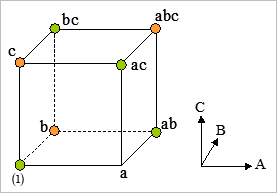
Figure 21.139 The geometric view of a \({{2}^{3}}\) design