20.6.5.2. Discrete Time Integrator

The Discrete-Time Integrator block implements discrete-time integration or accumulation of the input signal. The block can integrate or accumulate using the Forward Euler, Backward Euler, and Trapezoidal methods. In integration mode, \(T\) is the block’s sample time. In accumulation mode, \(T=1\). The block’s sample time determines when the block’s output signal is computed.

• Forward Euler method: \(\frac{1}{s}\) is approximated by \(\frac{T}{(z-1)}\).

  The output signal at step \(n\) is defined by \(y(n)=y(n-1)+T\times u(n-1)\)

  Let \(x(n+1)=x(n)+T\times u(n)\).

  At first step, \(\begin{aligned} & y(0)=x(0)\,\,\,\,\,Initial\,\,Condition \\ & x(1)=y(0)+T\times u(0) \\ \end{aligned}\).

  At second step, \(\begin{aligned} & y(1)=x(1) \\ & x(2)=x(1)+T\times u(1) \\ \end{aligned}\).

  At k-th step, \(\begin{aligned} & y(k)=x(k) \\ & x(k+1)=x(k)+T\times u(k) \\ \end{aligned}\).

• Backward Euler method: \(\frac{1}{s}\) is approximated by \(\frac{Tz}{(z-1)}\).

  The output signal at step \(n\) is defined by \(y(n)=y(n-1)+T\times u(n)\)

  Let \(x(n+1)=y(n-1)\).

  At first step, \(\begin{aligned} & y(0)=x(0)\,\,\,\,\,Initial\,\,Condition \\ & x(1)=y(0) \\ \end{aligned}\).

  At second step, \(\begin{aligned} & y(1)=x(1)+T\times u(1) \\ & x(2)=y(1) \\ \end{aligned}\).

  At k-th step, \(\begin{aligned} & y(k)=x(k)+T\times u(k) \\ & x(k+1)=y(k) \\ \end{aligned}\).

• Trapezoidal method: \(\frac{1}{s}\) is approximated by \(\frac{T(z+1)}{2(z-1)}\).

  Let \(x(n)=y(n-1)+\frac{T}{2}\times u(n-1)\).

  If \(T\) is fixed, the block uses the following steps.

  At first step, \(\begin{aligned} & y(0)=x(0)\,\,\,\,\,Initial\,\,Condition \\ & x(1)=y(0)+\frac{T}{2}\times u(0) \\ \end{aligned}\).

  At second step, \(\begin{aligned} & y(1)=x(1)+\frac{T}{2}\times u(1) \\ & x(2)=y(1)+\frac{T}{2}\times u(1) \\ \end{aligned}\)

  At k-th step, \(\begin{aligned} & y(k)=x(k)+\frac{T}{2}\times u(k) \\ & x(k+1)=y(k)+\frac{T}{2}\times u(k) \\ \end{aligned}\)

  If \(T\) is variable, the block uses the following steps.

  At first step, \(\begin{aligned} & y(0)=x(0)\,\,\,\,\,Initial\,\,Condition \\ & x(1)=y(0) \\ \end{aligned}\).

  At second step, \(\begin{aligned} & y(1)=x(1)+\frac{T}{2}\times (u(1)+u(0)) \\ & x(2)=y(1) \\ \end{aligned}\).

  At k-th step, \(\begin{aligned} & y(k)=x(k)+\frac{T}{2}\times (u(k)+u(k-1)) \\ & x(k+1)=y(k) \\ \end{aligned}\)

Dialog box

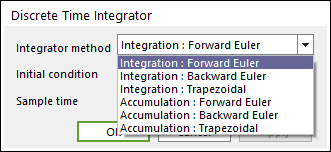
Figure 20.73 Discrete Time Integrator dialog box

Table 20.39 Parameters

Parameter(s)	Description
Integrator method	Select an integration or accumulation method.
Initial condition	If Initial condition source parameter is set to internal, the block gets initial conditions from this parameter.
Sample time	Enter the time interval between samples.

20.6.5.2.1. Example

Loan amortization model

In this example, we builds a CoLink model for the amortization of an automobile loan. At the end of each month, the loan balance b(k) is the sum of the balance at the beginning of the month [b(k-1)] and the interest for the month [ib(k)], less the end-of-month payment p(k). Thus, the balance at the end of month k is

\(b(k)=b(k-1)+\int_{T(k-1)}^{T(k)}{\left[ ib(k-1)-p \right]}dt\)

Examining the integrand, we can see that this problem can be solved using forward Euler integration. The below figure shows the CoLink model revised to use a Discrete-Time Integrator block with Integrator method set to Forward Euler. The Discrete-Time Integrator block Initial condition is set to 15,000 and Sample time to 1. Note that, in this case, the feedback gain is set to 0.01. Also note that the simulation End time must be set to 101, because the forward Euler integrator evaluates the rate at the beginning of a period.

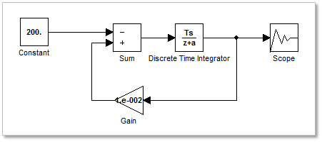
Figure 20.74 colink model

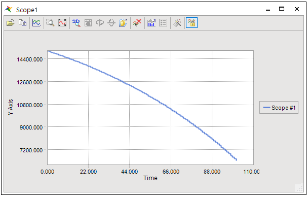
Figure 20.75 A result from scope